// classification problems

Support Vector Machines

Support Vector Machine is a type of machine learning model popularly used for solving classification problems. SVM is a linear classification technique that can only classify binary problems (i.e. where the Y variable has only two categories). In this article, SVM will be understood with a brief understanding of the mathematics behind it.

Understanding SVM Visually

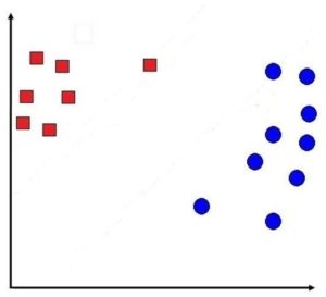
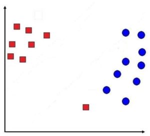
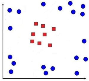
Before understanding SVM, let us understand how a linear classification model works. Suppose we have a dataset with the Y variable having two categories: 1 and -1. Below the -1 data points are shown in Red Squares while the 1 data points are shown in Blue Circles.

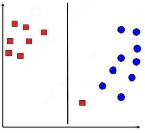
Now a linear classification technique uses a decision boundary (a line, in case of 2 dimensions, or a hyperplane, in case of a multi-dimension problem) to classify the data points.

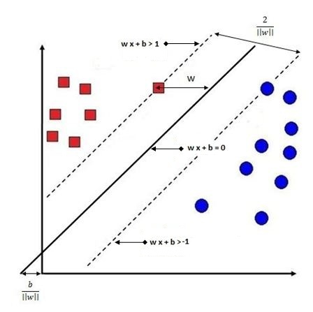
The equation for every hyperplane is w·x + b = 0.

To correctly classify the data, let’s say for input x_i, it should give us a value of w·x_i + b > 0 if Y_i = 1 (i.e. the equation should provide us with a value greater than 0 if the corresponding label is positive (1)). Similarly, the equation of the hyperplane, for an input of x_i, should give us a value of w·x_i + b < 0 if Y_i = -1 (i.e. the equation should provide us with a value lesser than 0 if the corresponding label is negative (-1)).

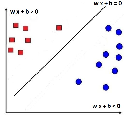
With all these equations what we mean is that if the value obtained from the equation is less than 0 then the datapoint will lie below the hyperplane (and will be classified as a red square), while if the value is greater than 0 then the datapoint will lie above the hyperplane (and will be classified as a blue circle). All this information can be summarised in an equation:

Y_i(w·x_i + b) > 0

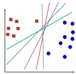
Now we come back to SVM. As shown above, multiple lines can be drawn to separate the two classes, but the question remains: which is the best line to classify the data points? Unlike other linear techniques such as the line of best fit used in linear regression, which can be found using a technique known as Ordinary Least Square Error, SVM uses a different method to come up with its decision boundary, where instead of simply coming up with a hyperplane to divide the data points, it uses margins to decide where the decision boundary should be created.

Let’s first understand this intuitively. Rather than using all the data points, SVM tries to maximise the distance between the two types of data points by increasing the margin, where the margin is the distance between the hyperplane and the datapoint lying nearest to the hyperplane.

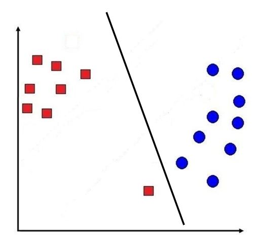
By doing so we are able to maximise the distance between the two types of data points, allowing better generalisation. In the below figure we use a straight decision line (dotted line). Notice how using such a line can cause a data point to be misclassified as a circle when it should have been a square.

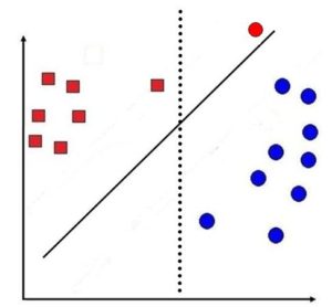
However, when we use a decision line created using SVM, where it takes into consideration the distance between the two closest data points of different classes (solid line), the data point is classified correctly.

This method of using margin to come up with a decision line is known as the Maximizing Margin Linear Classifier. In the above example, we are able to come up with the decision line by using SVM, which here uses two support vectors. The Support Vectors are the data points on the basis of which the margins are created. In our example, we have two data points which we use to maximize the distance between the two kinds of data points.

Thus here we come up with a decision line that splits the data in a way that the two support vectors are as far away from the decision line as possible, thereby maximizing the margin.

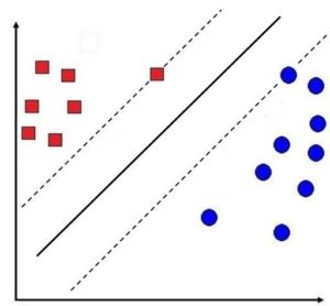
Intuitively we can say that to come up with a decision line using SVM, we can simply draw two margin lines on the data points of the two classes that are closest to each other, and then draw a decision line in the middle of these two margin lines.

Decision Line Mathematically

Coming up with the decision line is more complicated than what has been discussed so far, because SVM is a constrained optimization problem. The constraint is that the decision line should correctly classify the data points, so if the data point is -1 then it should lie below, and if it is 1 then it should lie above the decision line. However, we also want to optimize the model by maximizing the distance between the data points closest to this decision line.

To understand our constraint mathematically, we will write the equations mentioned earlier with respect to SVM.

Here the equation for the hyperplane is the same: w·x + b = 0.

However, instead of saying that for a value of x_i, w·x_i + b > 0 if Y_i = 1, we say that w·x_i + b ≥ 1 if Y_i = 1.

Similarly, w·x_i + b ≤ -1 if Y_i = -1. To make it more concise we can come up with an equation:

Y_i(w·x_i + b) ≥ 1.

This equation becomes our constraint. Now SVM will try to optimize by maximizing the margins while keeping in mind the constraint of correctly classifying the data points.

Now mathematically, the optimization problem boils down to calculating the margin by taking some arbitrary point on one margin to create the left margin, and adding some normal vector to it to bring us to the other margin, then calculating the distance, i.e. the length of that vector, and creating a decision line at half the distance of that added vector.

As mentioned above, we start with the left margin. Let’s say we have a data point on this margin which satisfies the equation: w·x_i + b + 1 = 0.

We add a normal vector to it (cw) so the equation becomes w·(x_i + cw) + b − 1 = 0.

Here c is the scalar which decides the magnitude of the vector being added to reach the next margin (the larger the value of c, the larger the margin it creates).

Now we put these two equations (w·x_i + b + 1 = 0 and w·(x_i + cw) + b − 1 = 0) together and come up with a new equation, which simplifies (after cancelling w·x_i and b from both sides) to:

w·cw = 2

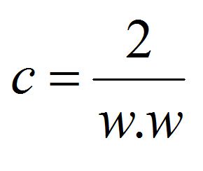
Now, this (c, scaled by w) is the margin, and we have to maximise it. Maximising this margin is equivalent to minimizing its reciprocal, which is the quantity below: this is our optimization objective.

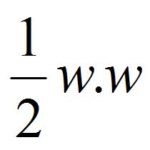
Now, to put the constraint and optimization together, we get: minimize ½w^Tw (i.e. maximise the margin) subject to the constraint Y_i(w·x_i + b) ≥ 1 (classify all the data correctly).

To do this manually we would have to find the values of w (the vector of coefficients) and b (bias/constant); however, this we will leave for the software to do.

Hard Margins V/s Soft Margins

When working on an SVM model, the practical question that arises is finding the optimal balance between the optimization and the constraint, because as we relax the constraint we can better optimize the model; however, relaxing the constraint too much will end up creating a weak model.

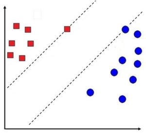
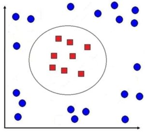
Let’s first understand this intuitively. For example, we have a dataset having data points as shown below:

If we create a decision line where the constraint is not relaxed (margins are not softened), then we will have a decision line where all the data points will be classified correctly, and the decision line created by SVM will look something like this:

This approach is the Hard Margin, as there is no scope for making any error. Such a method was developed by Boser in 1992 and can be used only when all the data can be classified linearly.

However, we can see that due to this we end up creating a narrow margin. And if we allow misclassification of one data point, we can come up with a margin which will be broader than the current one. This approach is known as the Soft Margin, where the constraint is relaxed and there is a scope for making errors. In such a scenario, the decision line would look something like this:

Thus we are able to maximise the margin by allowing some error to take place. Soft Margins can be used when the data cannot be separated linearly, and by allowing some error to take place we can maximise the margins. Soft margins were introduced by Vapnik in 1995. The benefit of such a method is that it helps in providing a model that generalizes well, which reduces overfitting.

However, making the margins too soft will cause the SVM model to underfit. This flexibility of choosing the softness of margins is controlled by C. C is the multiplier for the loss function, where the loss function is a way to penalize the misclassifications. Our optimization equation from before, ½w^Tw, will be called a regularizer here. We add a loss function (hinge loss function) to it, whose effect is controlled by using the multiplier C.

Therefore the higher the value of C, the more we penalize the model for making mistakes. Thus C acts as a tuning knob for the user to control the overfitting of the SVM model. A high positive value of C means pushing the model toward a hard margin.

(In SVM, the loss function is hinge loss, which can be written as (1 − y_i·(x_i,w))⁺. However this article will not get into the detail of the loss function.)

Thus, to understand the above equation in a different manner, we can say that the goal of SVM is to optimize the objective function, and the way we optimize is by minimizing the loss function. Thus we as users only have to take care of the C multiplier, which can be found by using methods such as grid search accompanied by cross-validation.

Kernel Trick

Suppose we have data that is not linearly separable, and using a soft margin will also not be feasible, as it will end up misclassifying a lot of data.

Here we have to use a non-linear classification technique, which is using SVM by applying the kernel trick.

This method was proposed by Vladimir Vapnik in 1992, where the dataset is transformed into a higher dimension where linear classification can take place.

Thus with the help of a kernel function, every dot product of input data points is mapped into the higher dimensional feature space by transformation.

There are many ways for such transformations, such as Linear, Polynomial, Sigmoid, Gaussian (Radial Basis Function), String, and Histogram Intersection, etc., with RBF being the most commonly used, having two common hyper-parameters to adjust: C and Gamma, where C is the multiplier of the loss function (discussed above), while Gamma is used to configure the kernel and is also used to control the complexity of the model, with a higher value of gamma making the model more complex, while a very low value will make the model underfit. Both these values can be found using grid search.

Thus the kernel trick is a great way of separating data which cannot be classified by the use of hard and soft margins.

Support Vector Machines is a very useful technique and works great for two-class classification problems, especially when the number of features is large and the dataset is small. However, its limitation is exposed when there is a multiclass classification problem. Also, SVM is sensitive to noise and becomes unreliable with an increase in the size of data. Also, the choice of kernel plays a crucial role when using the non-linear method, and often requires testing different models with different kernels, and overall this makes SVM a very computationally intensive algorithm. Nonetheless, it remains among the most effective ways to solve binary classification problems.