Time Series in R

Time Series models are used for forecasting values by analyzing the historical data listed in time order. This topic has been discussed in detail in the theory blog of Time Series. To demonstrate time series model in R we will be using a dataset of passenger movement of an airline.

Preparation

Importing Dataset

We will import the above-mentioned dataset using read_excel command.

library(readxl)
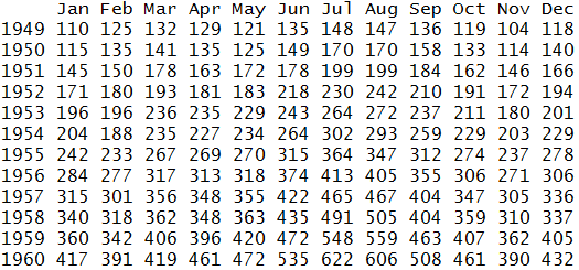
time <- read_excel('C:/Users/user/Desktop/Data Sets/Time_Series/AirPassengersData.xls')

Indexing Data

We will now convert our variable into R Time series objects using ts function. In the following function, frequency defines the number of observations per unit time. It will be equal to 4 for quarterly, 12 for monthly and so on.

time_passengers <- ts(time$`No. of Passengers`, start=c(1949,1),
end=c(1960,12), frequency=12)

We can now view the indexed data.

print(time_passengers)

Graphical Representation

To see the type of dataset we will use the above-indexed output to plot the graph. This graph is used to see trend or seasonality in our dataset.

plot(time_passengers,col='dodgerblue3',lwd=2)

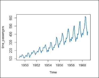
Air passengers time series plot showing trend and seasonality

Clearly, it's a trend and seasonal graph. Let us now look at different techniques for predicting the number of passengers for the next 12 months.

Averaging Techniques

There are mainly three types of averaging techniques - Simple Average, Moving Average and Weighted Average. These methods have been discussed in detail in the theory blog of Averaging Techniques. We will now demonstrate the Moving Average Technique using R.

Moving Average Technique

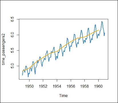
We can compute moving average using the aggregate function in R. This will compute average using the data for the previous one year and plot the graph for the same. First, we will convert the data to log values to eliminate trend/seasonality. This is done in order to forecast the values for future months.

time_passengers2 <- log(time_passengers)

Using aggregate function to compute moving average.

moving_avg <- aggregate(time_passengers,FUN=mean)
plot(time_passengers,col='dodgerblue3',lwd=2)
lines(moving_avg,col='orange',lwd=2)

Smoothing Techniques and Time Series Decomposition

Seasonal Trend Decomposition

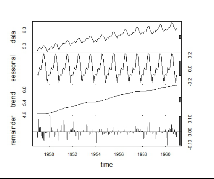
We will use stl function for decomposition. This will deconstruct the time series into three components namely trend, seasonality and remainder.

stl_passengers2 <- stl(time_passengers2,s.window="periodic")

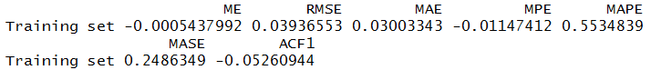
Checking Accuracy of the Model (STL Function-Decomposition)

Here, we compute the accuracy for the forecast model generated using STL function. We first start off by importing forecast library.

install.packages("forecast")
library(forecast)

Accuracy for All Variables

Here h is the number of periods for forecasting.

accuracy(forecast(stl_passengers2, h=12))

Plotting Graph

After computing accuracy of the model of STL function, we plot the STL components generated for each variable.

plot(stl_passengers2,lwd=1)

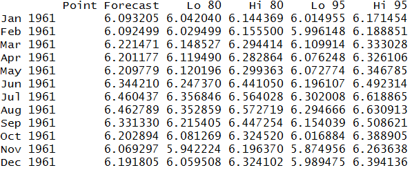
We will now make use of the forecast function for forecasting variables.

require(forecast)
forecast(stl_passengers2, h=12)

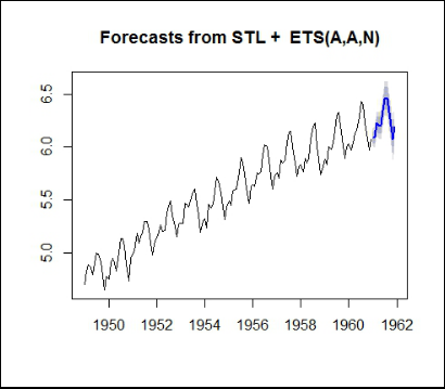
Graphical Representation of Forecasted Variables

We will now plot the above output.

plot(forecast(stl_passengers2, h=12))

Exponential Smoothing

ets function is used to fit exponential smoothing models.

ets_passengers2 <- ets(time_passengers2)

Calculating accuracy of ets for each variable.

accuracy(ets_passengers2$fitted,time_passengers2)

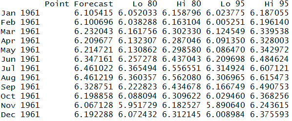
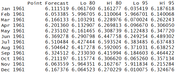
Now we will forecast using ets outputs.

forecast(ets_passengers2,h=12)

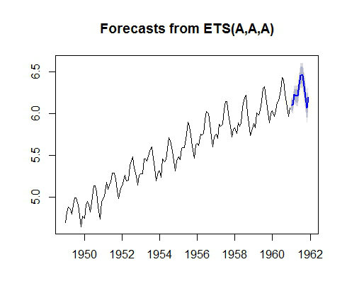
We plot the forecasted values by ets function (Smoothing Technique).

plot(forecast(ets_passengers2,h=12))

ARIMA Models

Initializing ARIMA Model

An automated way of forecasting is by using ARIMA models. Note that in R, we are using an automated ARIMA and hence don't specify the order tuple p,d,q which is Number of AR (Auto-Regressive) terms (p), Number of MA (Moving Average) terms (q), Number of non-seasonal Differences (d) like we did in Python. ARIMA is a function of forecast package.

arima_passengers <- auto.arima(time_passengers2)

Accuracy Score of ARIMA Models

Let us now compute the accuracy score of ARIMA models.

accuracy(arima_passengers)

Forecasting Using ARIMA Model

We will now forecast values for each variable using ARIMA model.

forecast(arima_passengers,h=12)

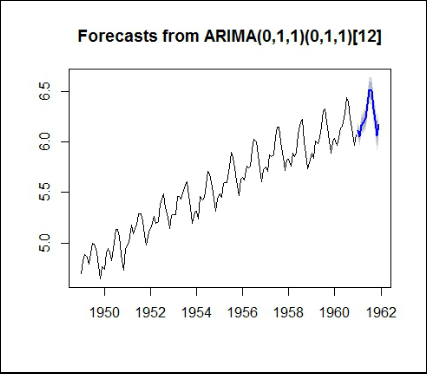
Finally, we represent the graphs for forecasted values from ARIMA model.

plot(forecast(arima_passengers,h=12))

In this blog post, many of the forecasting techniques were explored. The same techniques have also been explored in the blog Time Series in Python.