// time series

ARIMA Family

ARIMA stands for Auto-Regressive Integrated Moving Average. It is a high-level technique that is used for forecasting. Like ETS, ARIMA also requires the data to be stationary, and if the data is not stationary then the data is converted to make it stationary. ARIMA is specified by three order parameters known as p, d, q where AR is represented by p, I is represented by d and MA is represented by q. The ARIMA method is also known as the Box-Jenkins procedure (the process of fitting an ARIMA model is called so). ARIMA is a stochastic process, i.e. the data needs to be stationary so that its properties remain unaffected by a change in time.

There are various types of methods that fall under the ARIMA family, and they have been briefly explored below.

Auto-Regressive (AR)

In this method, the future value depends on the previous value, which can be mathematically denoted as:

Y_t = c + a₁Y_t−1 + e_t, −1 < a₁ < 1

Here the auto-regressive parameter p is used to specify the number of lags used (the number of past values to be taken) while applying the model.

The mathematical equation for the AR process is:

Y_t = c + a₁Y_t−1 + a₂Y_t−2 + a₃Y_t−3 . . . a_pY_t−p + e_t

Moving Average (MA)

Here the forecasted value depends on the previous error values, i.e.

Y_t = c + e_t − b₁e_t−1, −1 < b₁ < 1

The parameter q determines the number of terms to include in the model, i.e. how many past errors are to be taken while computing the forecasted value, which makes the equation for the Moving Average process look like:

Y_t = c + e_t − b₁e_t−1 + b₂e_t−2 + b₃e_t−3 . . . b_qe_t−q

Auto-Regressive Moving Average (ARMA)

This process can only be used when the data is stationary. This method is a combination of AR and MA, and when these two methods are used simultaneously, we get ARMA. Here two parameters are used: p to specify the number of lags, and q to specify the number of terms.

Auto-Regressive Integrated Moving Average (ARIMA)

ARIMA is an extension of ARMA, where ARMA can only be used on stationary data while the ARIMA model can fit on non-stationary data. This can be done through a method called differencing, which is used to make the data stationary. Here we introduce an additional parameter d, which determines the number of times we require to difference the data to make it stationary. The ARIMA model is a non-seasonal model which uses all three components - Auto-Regressive (p), Differencing (d) and Moving Average (q) - to create the non-seasonal ARIMA model.

When all three are combined, the mathematical equation for the ARIMA process comes out to be:

Y_t = c + a₁Y_t−1 + a₂Y_t−2 + a₃Y_t−3 . . . a_pY_t−p + e_t − b₁e_t−1 + b₂e_t−2 + b₃e_t−3 . . . b_qe_t−q

It is important to note, when using ARIMA, that if any of the parameters (p, d, q) is zero, then the de facto method being used changes, as we technically drop that component from the model. For example, if in our ARIMA model the value of p is 2 while the value of d and q is 0, then the method being used is simply Auto-Regressive, as the differencing and moving average components are missing.

Determining Stationarity of the Data

As mentioned above, the prerequisite for ARMA is that the data should be stationary. By stationary, what is meant is that the data should not have any trend, i.e. there is constant mean, variance and autocovariance over time. The data needs to be stationary for ARMA, as previous values determine the behaviour of the process for both AR and MA. Therefore we require data whose properties are constant over time, and thus the prerequisite becomes the data being stationary.

A typical line graph of stationary data looks something like this:

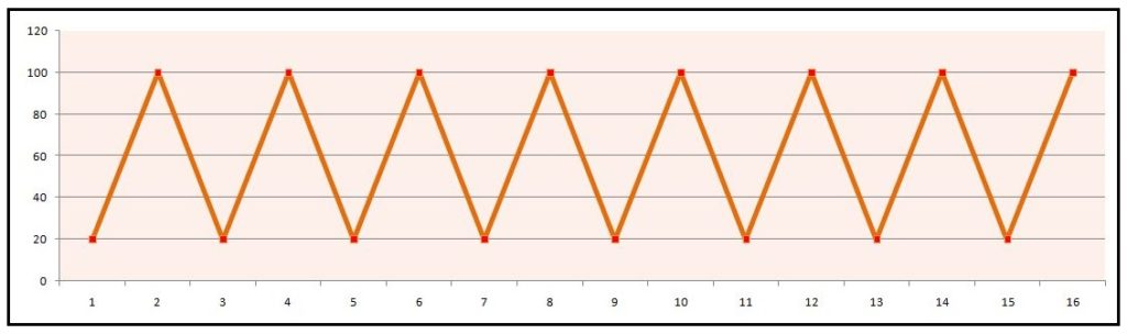
Here the data fluctuates with constant mean and standard deviation while there is no trend.

Note that irregularity is present even when the trend component is missing, and this cannot be considered as data being stationary, as different fluctuations among different time points cause irregularity, and this variance needs to be regular.

Thus a very simple way of determining whether the data is stationary or not is by simply looking at the graph.

Augmented Dickey-Fuller

Another method is by performing an Augmented Dickey-Fuller (ADF) Test, which is a statistical test where the null hypothesis states that the data is non-stationary while the alternative hypothesis states that the data is stationary. This test is also called the Unit Root test. Other methods include the KPSS test, etc.

Auto Correlation Function (ACF) and Partial Correlation Function (PACF)

Another method of defining whether the data is stationary or not is by finding the trend component through methods such as Auto-Correlation Function (ACF) and Partial Auto-Correlation Function (PACF).

Auto Correlation Function (ACF)

As mentioned in the previous blog, the trend is simply denoted by the regression line. For example, if we have a Price variable and 20 time periods, then we need to find, for a unit increase in the time period (if we move from time period 1 to 2), how much increase there is in the price. Thus, in a way, we do regression, i.e. for one unit of x, what is the change in y. Therefore the trend is nothing but the beta component in a linear equation. Thus we compute a linear trend where the current value of the variable 'price' is a function of the previous value of 'price'. Here we can see a concept of auto-correlation emerging. If we look at the below dataset with the time periods M1, M2, M3 . . ., as per autocorrelation we can say that M2 is a function of M1, M3 is a function of either M2 or M1, and so on. With this understanding, we come up with the concept of lag, where for Lag 1 we consider the previous value, for Lag 2 the value previous to the previous value, Lag 3 the value previous to that, and so on.

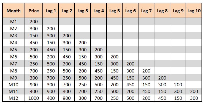
If we calculate the correlation between the Price and the lags (for example correlation(Price, Lag 1), (Price, Lag 2) . . . (Price, Lag 10)), then ideally the output should show a gradual decrease. If the correlation values peak at certain lags (for example a peak at every 12th month, which means the correlation is almost the same for all the Decembers), then it indicates seasonality. Thus this correlation between the variable and its lags is called the Auto-Correlation Function. ACF describes the strength of the relationship between different data points in the dataset. We can plot ACF and come up with correlograms, which are useful in determining the order of differencing (d) as well as the order of the moving average (q).

Partial Auto-Correlation Function (PACF)

This method provides us with the correlation between a variable and its lags which is not explained (affected) by previous lags. In the context of our example, if Price and Lag 1 are related, then Lag 1 and Lag 2 are also related. Therefore Lag 3 is impacting Lag 2, Lag 2 is impacting Lag 1, and Lag 1 is affecting sales, and so on. Now if we want to know the actual impact of Lag 1 on sales, there is a need to remove the effect of Lag 2 on Lag 1. Therefore, if we remove the previous value (Lag 2) and then calculate the correlation, this method is known as Partial Auto-Correlation Function. This method is used because we want to understand the effect of that particular time period alone, so if we don't know the past data and concentrate only on a particular time period, how much effect do we get. Like ACF, we can plot PACF, which can be used to help us determine the order of the auto-regressive parameter (p).

Methods of Making Data Stationary

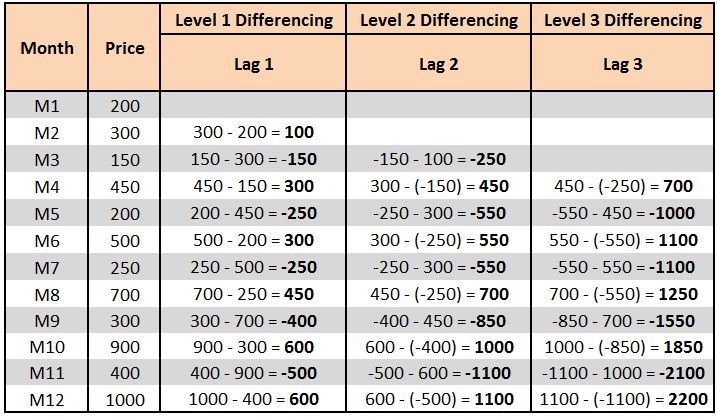
There are multiple ways of making the data stationary, among which the most common is through log transformations, which may help in stabilizing a strong trend. Another effective way is detrending, where we take the difference in the series, which helps in removing its trend from the data. What we require to know is how many times we need to do 'differencing' to make the data stationary. This provides us with the value of parameter d (the I of ARIMA). Therefore, if d is 0, then we don't need to do differencing, because the data is stationary and we can proceed with ARMA only.

Below we perform 3-level differencing, wherein in Level 1 we calculate the difference by subtracting the current period's value from the previous period's value. In Level 2 we include the second lag of the series, and so forth.

Overview of the Steps

A typical process of fitting an ARIMA model through the Box-Jenkins methodology includes:

Plotting data to see if any trend, seasonality or cyclicity is present. Decomposing the data to find the Trend, Seasonality, Cyclicity and Irregularity components (explored in the previous blog). Checking for stationarity by using methods such as the Augmented Dickey-Fuller (ADF) test, or by using ACF and PACF plots to know the order of differencing needed. If stationarity is not found, using transformations. If stationarity is still not achieved, finding the order of differencing using ACF and PACF plots and executing differencing to make the data stationary. Using ACF and PACF plots to find the order of AR and MA. Fitting the ARIMA model. Evaluating the model.

In application, the values of the parameters p, d, q can be found by the software alone, while determining whether the data is stationary or not, and making it stationary, can be done in software with simple one-line codes. One must remember the important difference between smoothing and ARIMA, which is that while both require the data to be stationary, smoothing techniques (for example, single exponential smoothing) take one past value and one past error value, similarly double exponential takes two of each, however in ARIMA we don't know in advance how many past values are to be taken, and also here the past value count and past error value count can be different - for example, we can take two past values while considering three error values.

ARIMA is a very powerful forecasting tool; however, when using this method, we must have a decent amount of data. It also generally works better on long, stable series of data. It is among the most advanced methods of forecasting discussed so far and must be used for precise forecasting.