// descriptive statistics

Measures of Shape

Measures of Shape as a descriptive statistics provide us ways to understand how the data points in a dataset are distributed and help us to understand the patterns that may be concealed and can be understood once the data is plotted on the graph. In this blog, the data along with the various shapes that it can have are explored. It is important to note that the shape of only a certain kind of data can be explained such as that of quantitative data that follows a logical order and have some sort of ‘weight’ whereas Qualitative data cannot be used, as its values don’t have any ‘weight’ to them.

The shape of the data can be understood by considering how the data points are distributed in the space. This distribution can be categorised into Symmetrical Distribution (e.g. Normal Distribution) and Asymmetrical Distribution (Skewed Distribution). In this post, each of such distributions are explored.

Symmetric Distribution

A Distribution can be called Symmetrical when the two sides of the distribution are a mirror image of each other, so if you separate the distribution from the mean, what you see on the left side of the distribution is exactly what you see on the right side of the distribution.

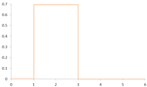
Examples of Symmetric Distributions are U-shaped distribution, Rectangular Distribution, Normal Distribution etc.

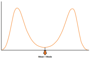
Most of the Symmetric Distributions are unimodal i.e. they have one peak, while the other kind is of bimodal or multi-modal where there is more than one peak in the distribution which is because there is more than one mode in the dataset, however, the mean and the median are same in such distributions. In this blog post, however, only one kind of Symmetric Distribution is discussed which is the Normal Distribution.

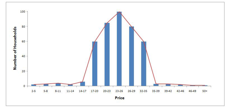
Normal Distribution

A Normal Distribution is a kind of a Symmetric Distribution where the mean, median and mode coincide with each other. The key features to identify a normal distribution or the characteristics that make a distribution ‘Normal’ are as follows-

Firstly- It is symmetrical, as explained above, the left and right side of the distribution are mirror images of each other when the distribution is divided from the middle where the mean, median and Mode coincide.

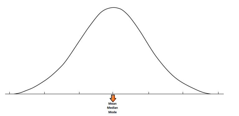
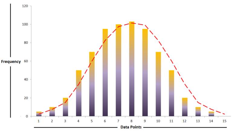
Secondly- Mean, Median and Mode coincide at the centre when such a data is plotted on a graph and because such a distribution is highest in the middle, it has a bell-shaped curve when a histogram is constructed. Such a distribution is unimodal i.e. there is only one value that gets repeated the highest time.

Lastly- The tails of the curve (upper and lower tails) never touch the baseline (x-axis) making the distribution asymptotic.

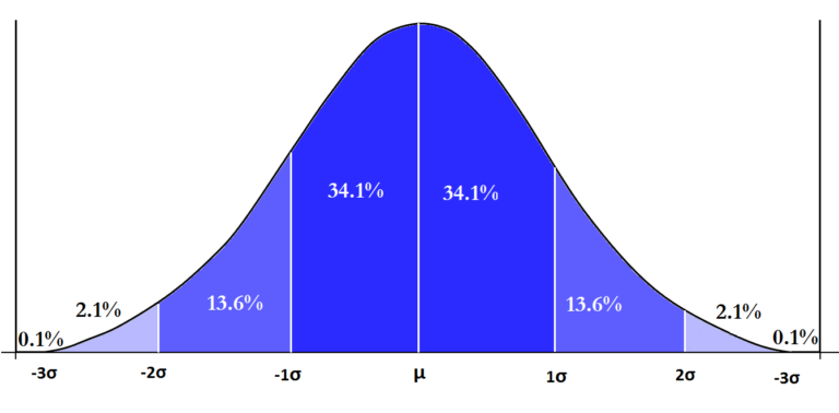
Each of these three characteristics of the normal distribution is very critical in statistics as they allow us to compute probabilities and also play a major role in Inferential Statistics. When all these 3 characteristics are taken into account, we can draw some conclusions such as that most of the data is around the centre and the values get perpetually extreme and rare when we move away from the centre on either of the sides. This brings us to the Empirical Rule or the Three Sigma Rule that allows us to say that when the data is normally distributed then 68% of the values lie within one Standard Deviation (the data above and below a unit of standard deviation is the same as the curve is symmetrical), 95% at 2 and around 99.7% at 3 Standard Deviations.

Asymmetric Distribution

If the collected sample data is systematically biased and includes data points that have certain particular characteristics then this causes the distribution to become asymmetrical. In Asymmetric Distribution, the two sides do not mirror each other.

Skewed Distribution

Skew is a characteristic often used to describe the distribution of values and in Asymmetric Distributions, the distribution can be skewed either Positively or Negatively and this happens when the more frequent values get cluttered around the high or low ends of the x-axis. Such a shape is one of the most common shapes when a distribution deviates from the normal distribution. In such a situation the mean, median and mode do not coincide with each other. The easiest way of identifying whether a distribution is skewed or not is to construct a histogram and look at the shape of the distribution. If it is skewed then it can either be a Positively or can be a Negatively Skewed Distribution.

Positively Skewed Distribution

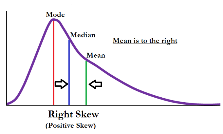
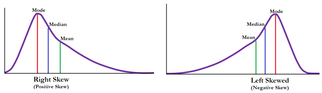
A distribution becomes Positively Skewed when the mean of the distribution is higher than the median and most of the scores occur at the lower end of the distribution while few scores are at the higher end. Any Probabilities based on such a distribution will underestimate the actual number of scores at the lower end of this skewed distribution while overestimating the number of scores at the higher end of the distribution. If we plot such a distribution on a histogram then the tail on the right side of the histogram is longer than the left side with the mean being on the right and median on the left and is the reason that Positively Skewed Distribution is also known as Right Skewed Distribution. Therefore the distribution is Positively Skewed when the mean is greater than the median (making mean to be on the right of median), few scores are at the low end creating an elongated tail at the higher end of the distribution.

Negatively Skewed Distribution

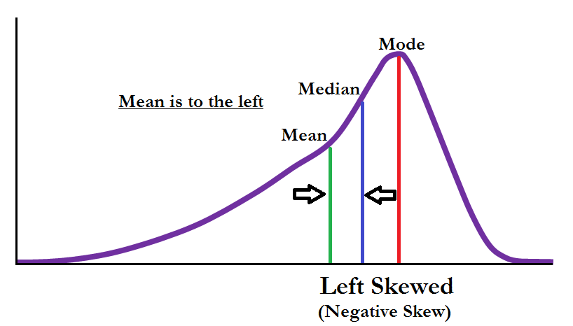
A distribution is Negatively Skewed when the median of the distribution is higher than the mean and most of the scores occur at the higher end of the distribution while few scores are at the lower end. Any Probabilities based on such a distribution will overestimate the actual number of scores at the lower end of this skewed distribution while underestimating the number of scores at the higher end of the distribution. If we plot such a distribution on a histogram then the tail on the left side of the histogram is longer than the right side with the mean being on the left and median on the right and is the reason that Negatively Skewed Distribution is also known as Left Skewed Distribution. Therefore the distribution is Negatively Skewed when the mean is smaller than the median (making mean to be on the left of median), few scores at the high end creating an elongated tail at the lower end of the distribution.

Typical Examples of skewed distribution can be of a surprise test of maths which if turns out to be very tough, causes a lot of students in the class to not score good marks and when the marks of such students are plotted, the shape of the distribution will indicate a Right-Skewed distribution. On the other hand, if the exam turns out to be very easy and all the students score extremely high marks then such a distribution will be a Left Skewed Distribution.

Other Shapes of Distribution

Apart from the Normal and Skewed, there are other shapes of distribution also which have been discussed very briefly below.

Kurtosis

Like skewness, Kurtosis is a descriptor of shape and it describes the shape of the distribution in terms of height or flatness. Some of the types of Kurtosis are Leptokurtic, Platykurtic and Mesokurtic.

Leptokurtic

When there is a positive excess of kurtosis, the shape of the distribution is called Leptokurtic. To understand this in terms of shape, it has fatter tails and if compared to a normal distribution it has a similar peak (to be precise, such a distribution has higher peak than what is found in a normal bell-shaped distribution and significantly higher if compared to a Platykurtic distribution) and has values clustered around the centre (mean).

Example- If you are asked to collect a sample to find out the average price of the car that people own in Delhi and you decide to go only in the upper-middle-class localities, then the shape of such a sample’s distribution will be Leptokurtic.

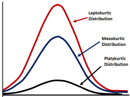
Platykurtic

When there is a negative excess of kurtosis, the shape of the distribution is called Platykurtic.

The data points are highly dispersed along the X-axis that results in thinner tails when compared to a normal distribution and has very few values clustered around the centre (mean). Such a distribution will have little central tendency.

Example- You are asked to go to 15 districts or localities of your city to collect a sample to find out the average income of the state. You decide to go to each district and find the average income of each district by randomly choosing 40 people and finding their annual income. But when the samples were finally plotted on a histogram, the shape of the distribution seemed to be Platykurtic, because all the 15 districts you chose to go were where government households were located where income of people fell in the middle-income band with all having more or less the same average income causing the shape of your distribution to become flatter than the normal.

Mesokurtic

This is when the distribution is normal. Here the tails of the distribution are neither too thin nor they are too thick and also the scores are equally divided with scores neither being clustered around the centre nor being too scattered.

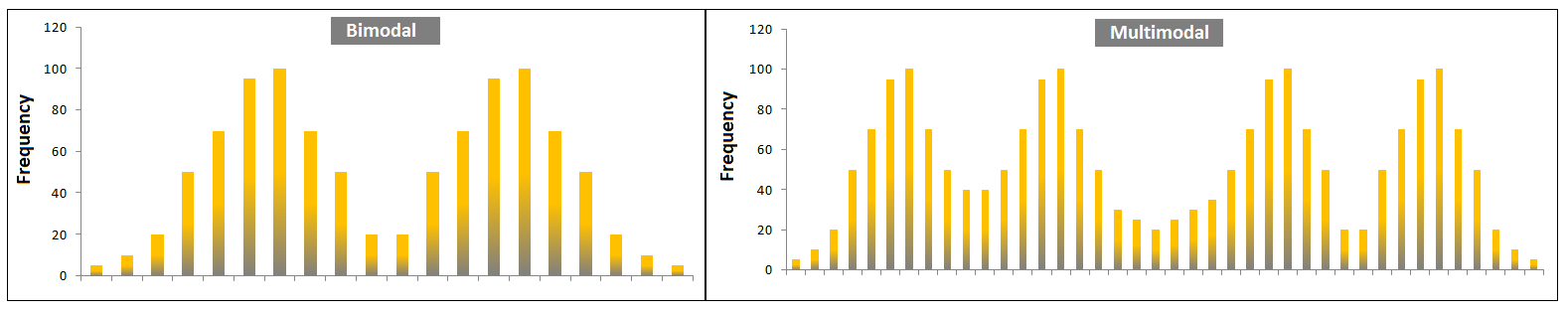
Bi-Modal and Multi-modal Distributions

A Typical normal distribution only has one peak. There can be a distribution which has more than one mode and in such scenarios, the distribution can be Bi-Modal (if there are two peaks) and multimodal (if there are more than 2 peaks). Such peaks may indicate different groups that might be present in the data or it may also mean that the data is sinusoidal (shape in the form of a wave).

The shape of distribution plays a very important role, as it is the shape of the distribution that makes it possible to draw inferences about the population from the sample data. Having a good understanding of the shape of the distribution is crucial in understanding how many inferential statistics work. In this blog post, what a normal distribution is and what other kinds of shapes a data can take other than the well-known bell-shaped curve etc were discussed. With the understanding of this section, you are ready to proceed to Inferential Statistics.