// descriptive statistics

Measures of Variability

Measure of variability describes how spread out a group of scores is, i.e. it helps us to describe the variability, how similar or varied the data points are in a sample or population.

Before understanding the different Measures of Variability, it is important to understand the need for a Measure of Variability when we have a Measure of Central Tendency at our disposal to describe and summarise our data in a single value. As discussed earlier, many of the Measures of Central Tendency suffer from outliers and the shape of the distribution and consequently fail to provide a correct and unbiased picture of the dataset. In addition to these, they also fail to make us understand how spread or scattered our data is and how far away they are from the "Centre".

Example

To understand this further we can take an example. If there are two buses in your locality, Bus-A and Bus-B, either of which you can choose to reach your school. You are supposed to reach your school at 8 o'clock with a scope of only 5 to 10 minutes to be late. Both the buses are available to you at roughly the same time, but the question is which bus should you choose to ride to reach your school on time. Hypothetically, we have the historical data of these two buses for the last 10 days where we find that both have an average of reaching the school at 8 o'clock.

Illustration of two school buses, Bus-A and Bus-B — Two buses, both with the same average arrival time.

A table of arrival times over 10 days for Bus-A and Bus-B, both averaging 8 o'clock — Arrival times over 10 days: same average, different spread.

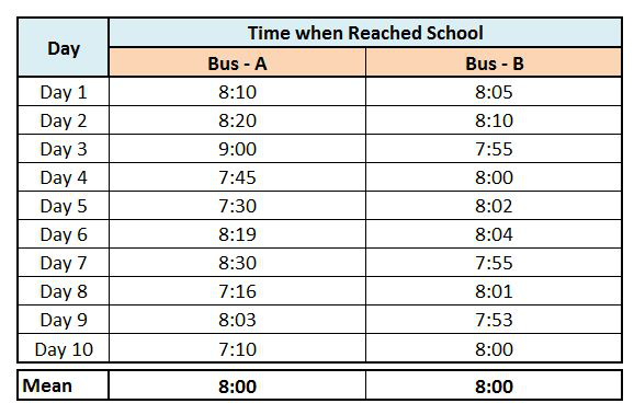
However, if we look closely, we find that Bus-A is way more inconsistent than Bus-B. The "Data Points" of Bus-A are way more "Spread Out" than those of Bus-B, making Bus-B more reliable. The Measure of Central Tendency, be it Mean, Median or Mode, fails to provide us with this critical piece of information, and this is where the Measures of Variability help us.

There are three main measures of Variability (Dispersion): Range, Variance and Standard Deviation. However, Standard Deviation is the one which is most commonly used.

Range

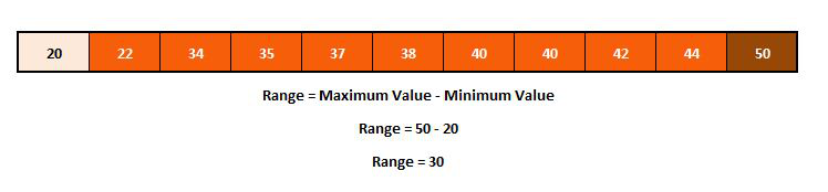
Range is simply the difference between the largest and the smallest value of our distribution or dataset.

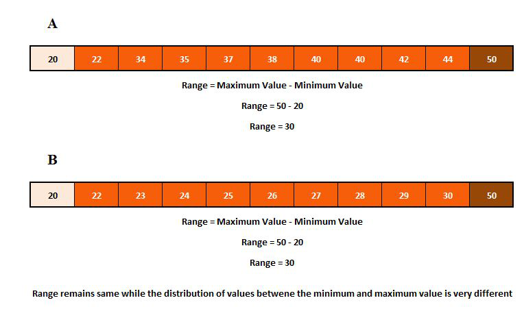
The problem with using range is that it can be quite misleading because it doesn't explain the spread between the minimum and maximum value.

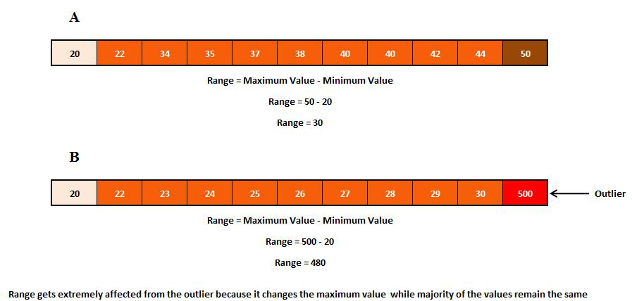
Two datasets with the same range but a very different spread of values between the extremes — Range remains the same while the distribution of values between the minimum and maximum value is very different.

Also, Range is highly vulnerable to outliers as it can change the minimum or the maximum value of the distribution.

Two datasets where adding a single large outlier dramatically increases the range — Range gets extremely affected by an outlier because it changes the maximum value while the majority of the values remain the same.

Quartiles

Quartiles, Quintiles, Deciles etc. can also be used as a measure of the range of scores in a dataset. Quartiles divide a dataset into 4 equal parts and refer to the values of the point between the quarters. The Lower Quartile (Q1) is the point between the lowest 25% of values and the highest 75% of values. It is also called the 25th percentile. The second quartile (Q2) is the middle of the dataset. It is also called the 50th percentile, or the median. The upper quartile (Q3) is the point between the lowest 75% and highest 25% of values. It is also called the 75th percentile.

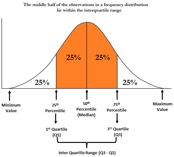
An Interquartile Range is the difference between the value that marks the 75th percentile (3rd Quartile) and the value that marks the 25th percentile (1st Quartile), unlike the Range which simply is the difference between the largest and the smallest value. If the values in a distribution are arranged from smallest to largest and are divided into 4 equally sized groups, then the Interquartile Range would be the values in the middle two Quartiles, describing the middle 50% of the values of the distribution. One of the advantages that Interquartile Range has over Range is that it is not affected by outliers, while Range can be adversely affected by Outliers.

Sum of deviation is always 0

For example, if we have a dataset with 4 values, 45, 64, 68, 51, having a mean of 57, and we try to find the "deviation" of each of these values from the mean by subtracting the mean from each of these values (45-57=-12, 64-57=7, 68-57=11, 51-57=-6) and try to summarise all this by adding the result values, then the outcome will be a useless 0 (-12 + 7 + 11 + -6). Therefore the sum of all these "deviations" is 0, i.e. the mean deviation from the mean is always 0. This happens because mean is simply the mathematical middle of the distribution and, naturally, some of the scores will fall above or below the mean and consequently produce negative and positive values of deviation, and when we sum all these together, the negative values cancel out the positive values leaving us with a 0. As we cannot find an average of 0, we use a different measure to counter this problem. We can use Mean Absolute Deviation (MAD) or the most commonly used Variance, which can produce Standard Deviation, to avoid getting a sum of 0 as our numerator when we try to divide the sum of our deviation by the denominator, the number of values in the observed distribution.

Mean Absolute Deviation (MAD)

To counter the above-mentioned problem, we take Mean Absolute Deviation, i.e. the average distance from the mean. We calculate Mean Absolute Deviation by subtracting the mean from each of the observations, summing up all these "distances" together (ignoring the signs, as Mean Absolute Deviation is calculated by only considering the absolute values so the output is always positive) and dividing it by the number of total observations. In our case, the MAD (Mean Absolute Deviation) comes out to be 9 (12+7+11+6=36, 36/4=9). Mean Absolute Deviation is useful as it is easy to understand and calculate, providing us with an average of deviation that can be found in our distribution, but it can be affected by extreme values which may cause the mean to change, on which it heavily relies. Also, it violates the algebraic principle by ignoring the + and − signs while calculating the deviations.

Variance

The variance, unlike Range and Interquartile Range, measures the spread of the data around the mean and explains how much each value in the data is close to the mean of the distribution. Variance is the average squared distance from the mean and is another measure to identify how close the scores are to the mean, i.e. the middle value of the distribution. It also counters the problem mentioned above where the mean deviation from the mean is always 0. To counter this problem we take the square of the deviation from the mean so that the result is not 0. For example, the Variance of the above-mentioned data set will be 87.5.

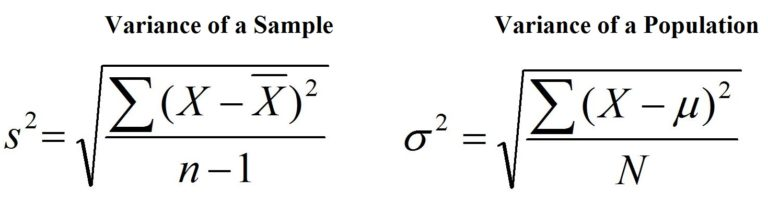
where Σ means to sum, X is a score in the distribution, μ is the population mean, N is the number of cases in the population, x̄ is the sample mean and n is the number of cases in the sample.

Standard Deviation

Variance, despite its uses, is often used only as a step in the calculation of other statistics and is generally not used as a stand-alone statistic. Variance is calculated as a step in calculating standard deviation, where we take the square root of the variance, mainly because the values have units and by taking squares of those units they may produce odd results. For example, if the unit of measurement of our values is in metres and we try to find out the variance of such a distribution, then the result will be in square metres. So, as we take the square so that the negative values don't cancel out each other, it is a good idea to normalise them back by taking the square root of the variance. Thus we get Standard Deviation by simply taking the square root of the Variance. Standard Deviation is often used as a yardstick to determine how much deviation from the mean is acceptable in a given distribution. Also, in certain scenarios, if there are two datasets with the same means and with different standard deviations, then one can say that the dataset with high standard deviation is more "unreliable" than the one with low Standard Deviation (as in the above example of two school buses). For example, the Standard Deviation of our above-mentioned data set will be approximately 9.35 (the square root of the variance, 87.5).

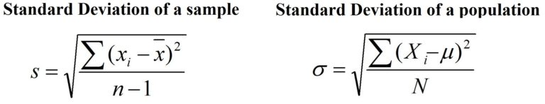
where Σ means to sum, X is a score in the distribution, μ is the population mean, N is the number of cases in the population, x̄ is the sample mean and n is the number of cases in the sample.

Sample vs Population Variance/Standard Deviation

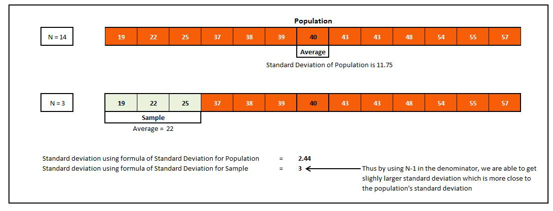
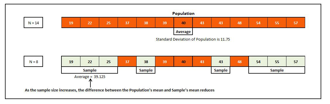
If you would have noticed, under Variance and Standard Deviation, two kinds of formulas are mentioned for each one of them. One is for the Population while the other one is for the Sample. The formulas for calculating variance and standard deviation depend on the kind of distribution you are working with. If the distribution scores are of a sample then there is a different formula, and if the scores belong to the population then there is a different formula. Explaining the reason briefly, it is mainly because both these Measures of Deviation, Variance and Standard Deviation, heavily rely on the arithmetic mean of the distribution, and any change in the mean directly affects their outcome. While the mean calculated from the population is the "Actual, True or Correct" mean as it is being calculated directly from the values of the actual population in question, the mean calculated from the sample of this population is merely an estimate of the actual mean (which is the population mean) and will be different from it. So if we use the sample mean and calculate the sum of squares of the sample variance, it will consequently produce a slight bias when we calculate the Variance or Standard Deviation. Since sample mean is calculated from the values of the sample distribution, which are on average closer to the sample mean than they would be to the population mean, they produce a smaller (biased) variance. To counter this bias we use a smaller number in the denominator, so rather than dividing the sum of squares of the sample variance by the number of cases in the sample (N), we divide it by a smaller number, i.e. N-1, so that we get a larger output (variance) as a result, countering the bias.

Comparing the standard deviation of a population against a sample, where dividing by N-1 gives a larger sample standard deviation closer to the population value — Using N-1 in the denominator gives a slightly larger sample standard deviation, closer to the population's standard deviation.

The formula for Population Variance/Standard Deviation should be used in calculating various statistics if the population mean is known, and the formula for Sample Variance/Standard Deviation should be used if the population mean is not known and is being estimated by using the mean of the sample. However, if the sample size is big enough (i.e. if we have a lot of data) then using either of the formulas to calculate statistics will be fine as the difference will be negligible, because the standard error reduces with the increase in the sample size. This can also be understood in terms of covering more of the population: when our sample size is large, we are able to get closer to the population's mean and the benefit from having N-1 in the denominator reduces.

As the sample size increases, the sample mean converges towards the population mean — As the sample size increases, the difference between the population's mean and the sample's mean reduces.

Thus Standard Deviation is one of the most important Measures of Variability out there. Unlike Mean Absolute Deviation, it follows the algebraic principles and considers the negative and positive values produced during the calculation of variance. It can be used for further algebraic treatment as well as for higher statistical analysis; however, it can get very much affected by the extreme values, as a square of the deviation of a disproportionately bigger value will produce a much larger output than those of smaller weight.

In this blog post, various ways were explored through which we can understand how our data is spread. The concepts of Measures of Central Tendency and Measures of Variability will help us in understanding the next blog, which is Measures of Shape, where the various shapes that the data can take, along with how these shapes help us in describing our data, are explored.