// classification problems
Artificial Neural Networks - Backpropagation
The single most important feature of Artificial Neural Networks that makes it a more efficient algorithm than others is its ability to minimize error through the use of Backpropagation. Artificial Neural Networks has been explored under the Modeling section, and in this article a mechanism known as the Backward Propagation of Errors with Gradient Descent is explored which makes ANN unique from other algorithms.
Derivatives
Backward propagation requires calculating error, which is done using an error function. For this, the gradient of the error function with respect to the weights of the neural network is calculated. The calculation of the gradient is performed from the back (from the output layer) to the front (the input layer). However, to understand how we derive the gradient, we should first understand how Gradient Descent works.
First, let’s start with an understanding of what we mean by a derivative. There are several ways of thinking about the derivative of a function, and the simplest way of describing the derivative of a function is when we imagine a function as a slope, where the derivative tells us how quickly the function is changing at a particular point.
Thus if we have a function f(x) at point x, then the derivative is simply the indication of whether the function will increase or decrease upon increasing x. In the image below we can see that at point x1 the derivative is positive, as upon increasing x1 the function will grow, while the derivative is negative at x2, as upon increasing the value of x2 the function will decrease.
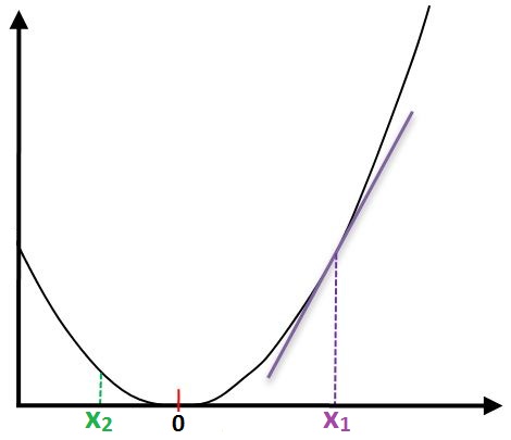
If we try to understand derivatives in the context of Backpropagation, then the above function is an error function. Here we need to understand derivatives in relation to the optimum value, where for the error function the optimum value is zero. Derivatives help us know whether our current value of x is lower or higher than the optimum value. Therefore, if we have x1, the derivative is positive, which indicates that x1 is bigger than the optimum value and should be decreased to reach the optimum value, while on the other hand, the derivative at x2 tells us that it is smaller than the required value and should be increased to attain the optimum value.
In Artificial Neural Networks we discussed how a model made up of a single neuron acts as a logistic regression (classification problem) or linear regression (regression problem), which becomes evident when comparing the equation of an artificial neuron, Y = wx + b, with that of Linear Regression, Y = mx + b. Therefore, let’s first take an example of Linear Regression, where the slope provides us with Y′, the predicted values. We can calculate the error by subtracting the actual value Y from the output Y′, i.e. the error is Y - Y′. This error can be plotted on a line graph, and this line can be described as an error function.
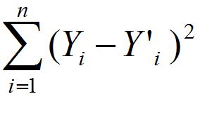
The cost function, aka loss function, provides us with all the error that our model has generated. The formula of the cost function is:
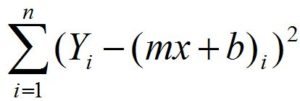
This equation can also be written by expanding Y′ as:
Our objective is to minimize this cost function, and this can be done by manipulating the values of m and b, as everything else is a constant. Our cost function is basically Y = x2 (here Y is our loss and x2 is our error), i.e. f(x) = x2, and as shown above, when plotted on a graph, we can take a point, e.g. x1, and find which direction to go to find the optimum value producing less error.
This decision of choosing the direction is taken through derivatives, where we draw a tangent line to the slope of the curve and calculate the derivative, and based on the value of the derivative we can decide the direction in which we need to move. However, we also have something known as the learning rate, which intuitively means how big a step we want to take in that direction in order to reach the optimum value. This whole process of using derivatives to minimize the cost function is known as gradient descent.
To minimize the error we need to find the optimum values of m and b, and need to find how the error changes with the change in m and b respectively. Thus our optimum value of m is m = m + Δm (here Δm, delta m, means the change in m), while the optimum value of b is b = b + Δb (here Δb, delta b, means the change in b).
As finding the derivative tells us which direction to move in order to minimize the error, we decide to find the derivative of the cost function. To do so, we simplify the cost function by removing the summation, as we have two ways of performing gradient descent: Batch Gradient Descent and Stochastic Gradient Descent. In the Batch method we consider all the inputs in a single go, while in Stochastic we compute the gradient using a single sample at a time. As we go for the stochastic approach here, we remove the summation and consider each error at a time. We also write Y - (mx + b) simply as ‘error’, which makes our cost function look like:
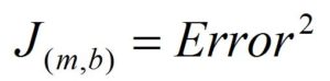
Here our cost J, which is a function of m and b, is equal to the square of the error. Now, to find the derivative of J relative to m, which basically means finding how J changes when m changes, we need to be clear on two more concepts related to calculus - the Power Rule and the Chain Rule.
Power Rule
If we have a function f(x) and it is equal to some power of x, i.e. xn, where n is not equal to 0, then the derivative of f(x) will simply be nxn-1. So if our function is f(x) = x2, then the derivative of f(x) will be 2x2-1, which is 2x1, which can simply be written as 2x. Similarly, when f(x) = x4, the derivative of f(x) will be 4x4-1, which equals 4x3.
Chain Rule
If we have a function x which is equal to y2, i.e. x = y2, and a function y which is equal to z2, i.e. y = z2, then as x depends on y and y depends on z, if we want to find the derivative of x relative to z we can find the derivative of x relative to y and then multiply it by the derivative of y relative to z. We can chain the derivatives together in order to find the derivative when they are not directly connected but are indirectly linked. Here, if we apply the chain rule, the derivative of x relative to y will be 2y, while the derivative of y relative to z will be 2z, making the derivative of x relative to z equal to 2y × 2z. We can also put this another way: if f grows a certain number of times faster than g (e.g. grows twice as fast as g), and g grows a certain number of times as fast as x (e.g. g grows twice as fast as x), then we can know how quickly f grows (here f grows 2 × 2 times as fast as x).
Backward Propagation Equation
Now coming back to:
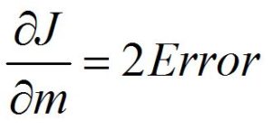
If we apply the chain rule, we know that for f(x) = x2, the derivative of x will be 2x. As we are trying to find the derivative of the cost function, which can simply be written as Error2, then as per the power rule, the derivative of the cost function is 2×Error.
Now we find the derivative of the cost function with respect to the error. However, we cannot simply stop here - we require the chain rule. We know that J is a function of Error2, while Error2 is a function of m and b. As per the chain rule, this makes the equation:
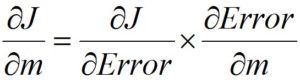
As we are looking for Δm, we apply the chain rule and try to find the derivative of the cost function relative to m, and for that we multiply the derivative of J relative to the error with the derivative of Error relative to m. To calculate the derivative of Error relative to m, we find the partial derivative, as Error is relative to both m and b, and as we are only focusing on m, we calculate partial derivatives.
We know that Error = Y - (mx + b), which can be written as Y - xm − b, and as we are computing the partial derivative, apart from m everything is a constant, which means x, b and Y are constant. By applying the power rule we can say that the derivative is 1 × x × m0, and as constants don’t change, their derivative is 0, which brings the derivative to simply the value of x.
Thus the derivative of J relative to m is 2 × error × x. We then multiply this by the learning rate to decide how far we want to go in the direction of the optimum value provided by the derivative, making the equation (2 × error × x) × learning rate. As our error and x will be multiplied by the learning rate, we can get rid of the 2 (removing the 2 and instead having 2 as part of the learning rate produces similar results and gives us more control over the process), making the final equation error × x × learning rate.
Similarly, the derivative of J relative to b is the derivative of J relative to the error multiplied by the partial derivative of Error relative to b, and as in the equation Y - mx − b, m, x and Y are constant, as per the power rule the value of the derivative comes out to be 1 (1 × b0 = 1). Thus the derivative of J relative to b comes out to be error × 1 × learning rate, i.e. error × learning rate.
Thus m = m + Δm, where Δm is error × input × learning rate, while b = b + Δb, where Δb is error × learning rate.
Understanding Backpropagation with an Example
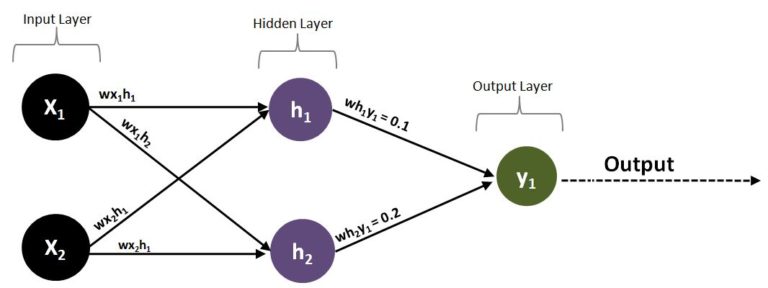
To understand backpropagation from scratch, we will start with a three-layer model where we have one input (x1), one hidden neuron h1, and one output y1. If we concentrate only on the weights between the hidden layer and the output layer, then we have one connection from h1 to y1 with weight wh1y1, which has a value of 0.1.
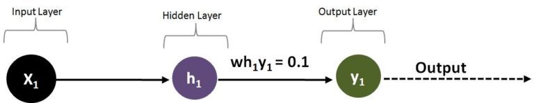
For a moment, presume that we had one input, which was used by the h1 neuron to generate a result that was passed to the y1 neuron, and after passing through the activation function gave an output of 0.6. As we are working in a supervised environment, we also have the correct labels to compare the result with. As per the correct label, the result should have been 1, which means we have an error of 0.4 (1 - 0.6). We can use this 0.4 (e1) to adjust the weight wh1y1 in order to produce a better result (i.e. less error). Here, as the output is less than expected, we should increase the weight in order to produce an output closer to 1 (note that we are not considering the influence of bias for now). Thus we increase the weight in the direction of the error in order to minimize the error.
Now, if we increase the number of neurons in the hidden layer by one and introduce another neuron h2, we will have another weight wh2y1, having a value of 0.2, and these two weights (wh1y1 and wh2y1) will be connected to the output neuron y1.
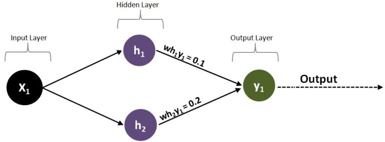
We will now be required to adjust two weights in order to minimize the error produced by y1; however, we don’t know which weight is responsible for the error or to what extent each weight is participating in producing the error. For this, we consider the size of the weight, which means the higher the weight, the more responsible it is for the error. Therefore, to adjust the weight wh1y1, we use the formula (wh1y1 / (wh1y1 + wh2y1)) × e1, and for wh2y1 we use the formula (wh2y1 / (wh1y1 + wh2y1)) × e1, which basically means that as wh2y1 has the higher weight (0.2), it is more responsible for the error - roughly two-thirds - while wh1y1 shares one-third of the responsibility for causing the error. Thus we will tweak the weight wh1y1 by 33% while the weight wh2y1 is adjusted by 67%. We adjust the ‘delta weights’ proportionately, based on the value of their weights, in order to minimize the error (e1).
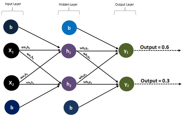
So far we have concentrated only on the second and third layers. If we add two neurons in the input layer, we create a structure similar to the multilayer perceptrons discussed under Artificial Neural Networks.
Now we have two inputs, x1 and x2. Thus we have four weights connecting the input layer to the hidden layer (wx1h1, wx1h2, wx2h1, wx2h2). It is important to understand that the error on y1 can be manipulated by tweaking the weights connecting the hidden and output layer; however, the neurons in the hidden layer are also directly affected by the neurons in the input layer, as a set of weights connects the input and hidden layers. Therefore, tweaking these weights changes the values of the hidden neurons, which in turn affects the output and the error. We therefore need to know in which direction, and to what magnitude, the weights of the input and hidden layer should be tweaked.
So far we tuned the weights of the hidden-output layer based on the error found at the output layer, and we could do so because they were directly connected, so we had an error we could calculate and assign responsibility for to different weights in order to adjust them. However, the weights of the input-hidden layer are not directly connected to the output layer, and thus we need to calculate the error of the neurons in the hidden layer in order to tweak the weights of the input-hidden layer.
Thus we see a backward mechanism at work, where the error at the output layer is used to tweak the weights of the hidden layer, while the errors at the hidden layer are calculated to adjust the weights of the input layer.
To adjust the four weights of the input-hidden layer (wx1h1, wx1h2, wx2h1, wx2h2), we need to calculate the errors on h1 and h2, which we have already done above, according to which the error on h1 is 33% while the error on h2 is 67%.
If we consider the model structure discussed under multilayer perceptrons and make it more complex by adding two neurons in the output unit, where y1 predicts the value 1 while y2 predicts the value 0 (a binary classification problem), we can see how complex backpropagation can become, as we now have two neurons in the output layer, y1 and y2, with y1 producing an output of 0.6, causing an error e1 of 0.4 (1 - 0.6), while y2 produces an output of 0.3, causing error e2 to stand at −0.3 (0 - 0.3). The number of weights has now increased from two (wh1y1, wh2y1) to four (wh1y1, wh2y1, wh1y2, wh2y2), and while the weights wh1y1 and wh2y1 should be increased to minimize e1, the weights wh1y2 and wh2y2 need to be decreased to minimize the error e2.
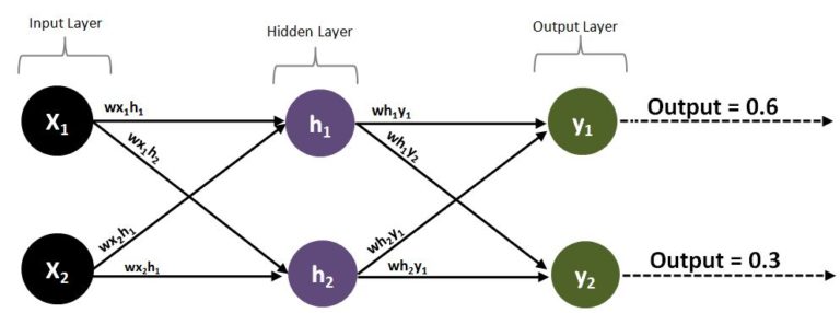
Therefore, the formula for calculating the error on h1 and h2 changes a bit, as we now have more weights (due to the increase in the number of neurons in the output layer) connecting the hidden and output layers:
Error h1 = ((wh1y1 / (wh1y1 + wh2y1)) × e1) + ((wh1y2 / (wh1y2 + wh2y2)) × e2)
Error h2 = ((wh2y1 / (wh1y1 + wh2y1)) × e1) + ((wh2y2 / (wh1y2 + wh2y2)) × e2)
The responsibility is thus taken on by each neuron in the hidden layer, as the error is calculated for each of these neurons by computing a proportion of the error with respect to their weights. Now that we have the errors of the hidden layer neurons, through gradient descent we can tweak the weights of the input-hidden layer, since we now have the required errors to perform the necessary calculation. Another way of looking at the above formula is that the denominator helps normalise these weights so they add up to 100%; however, as we will be multiplying all of this by a learning rate, we can get rid of the denominators, and as we are multiplying the error by the weight, the outputs will still be proportional. Thus the equations can be written as:
Error h1 = (wh1y1 × e1) + (wh1y2 × e2)
Error h2 = (wh2y1 × e1) + (wh2y2 × e2)
Updating the Weights and Biases
We can now start calculating the gradients. We know that if we look at each neuron individually, it has an equation similar to that of a linear regression, and above we calculated the derivatives for m and b. Drawing a parallel between linear regression and a single-neuron network, m can be written as w (weight) in the context of neural networks, so we will be finding Δw, while b (the bias term) remains b. However, we need to update the formulas, as we are now in a multidimensional scenario, and unlike linear regression, where Y = mx + b, here we have an activation function, sigmoid, which makes the equation y = σ(wx + b). We should also remember that we are now dealing with matrices, as we are in a multidimensional problem.
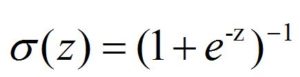
It is important to note at this stage that the sigmoid function is:
While the derivative of the sigmoid function is:

(which is basically the sigmoid times one minus the sigmoid).
Therefore, if we are looking to update the weights connecting the hidden layer and the output layer (wh1y1, wh2y1, wh1y2, wh2y2), the change in these weights can be represented by:
Δwhidden→output = learning rate × Error × H (the input provided by h1 and h2 to the output neurons) × the derivative of the output, i.e. σ(x)(1 - σ(x)).
Here we take the derivative of the output, as we have an activation function (in our example, sigmoid), and unlike linear regression, where there was no such thing, here we also need to calculate the gradient of it, which is the learning rate multiplied by the error of the output, multiplied by the derivative of the output. As we can presume the output has passed through the sigmoid, we can rewrite the equation as:
Δwhidden→output = Learning Rate × Error × (output(1 - output)) . HT
(We write H as HT because we transpose the input H, as it is a single-row matrix, and we need to transpose it before taking the dot product.)
We can similarly update the weights connecting the input and hidden layer (wx1h1, wx1h2, wx2h1, wx2h2), and here the errors will be the hidden layer errors (Error h1 and Error h2), while the inputs will be x1 and x2, and H (which was the input in the formula above). Thus the equation for updating these weights is:
Δwinput→hidden = Learning Rate × Hidden Layer Error × (H(1 - H)) . XT
We now move on to updating the biases, and for this, as mentioned earlier, we do not consider the input. Thus we get the following equations for updating the biases:
Δbhidden→output = Learning Rate × Error × (output(1 - output))
Δbinput→hidden = Learning Rate × Hidden Layer Error × (H(1 - H))
Backward propagation is among the aspects of Artificial Neural Networks that makes it distinct from other learning algorithms. Backward Propagation takes the error value and computes the partial derivative with respect to the weight and bias in each layer. This is done from the output layer to the input layer, i.e. recursively, and through this we are able to update the weights and biases and again run forward with the updated weights and biases, compute the error, and repeat the process until the minimum error is found. Thus we update the weights and biases through backpropagation in order to decrease the error in the output.