// regression problems

Linear Regression

Regression is a statistical method used to measure the relationship or quantify the association of independent variables with the dependent variable. In this article, we explore Linear Regression, where the relationship between the dependent and independent variable is linear. If the relationship between the variables is not linear, then other types of regression are to be used, but here, for using linear regression, we have to consider a very strong assumption that all the independent variables are linearly related to the dependent variable. Also, for linear regression to function, all the variables must be continuous (interval/ratio scaled).

Use of Linear Regression

Now, why is Linear Regression used when we have other statistical techniques? The answer is that building a linear regression model helps in answering much more complicated questions. Linear Regression helps in two ways. To explain this, two different scenarios can be considered.

Scenario 1: An automobile company wants to expand in your country and is searching for the city where it will open its first dealership. The company has data where, for various factors (independent variables), their corresponding sales are provided. Here Linear Regression can help, as it will be able to explain which factor plays the most important role in deciding the location of the showroom.

Scenario 2: An automobile company wants to launch a new variant of an already existing car. They want to know how much decrease in the price and increase in the mileage will make the car's sales double. Here Linear Regression can provide specific values, on the basis of which the company can set their price and initiate an engine refinement process to increase the car's mileage.

Thus, Linear Regression provides us with the variables that are important and also provides us with values through which these variables can be used to predict the dependent variable.

Types of Linear Regression

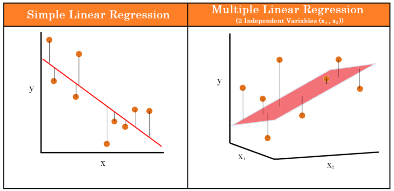
There can be two types of Linear Regression: Simple Linear Regression and Multiple Linear Regression. We first explain the statistical concepts through Simple Linear Regression, as 2-Dimensional scatterplots can be used to explain the calculation that a statistical software does in the backend while creating a Regression Model.

Simple Linear Regression

Simple Linear Regression can be performed when we have two variables, one dependent variable and one independent variable. For example, we have a dataset where the income of various car dealers is provided along with the number of cars sold at their showroom. Here our dependent variable is ‘Income’ while the independent variable is ‘Sales’. When we plot these two variables, it turns out that these two variables are positively correlated, and the value of Income is decided by the Sales.

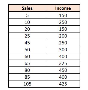
Table of Sales and Income values for various car dealers — Sales and Income data for various car dealers.

When plotted on a scatterplot, we get the following graph:

Scatter plot of Income against Sales showing a positive correlation — Income plotted against Sales.

In Simple Linear Regression, we cannot use Linear Regression to find the independent variables that are important, as there is only one independent variable involved; however, the other question, the predictive aspect, can be solved, where we can find that for a given value of Sales, how much Income can be expected. To find the predicted value, a regression line is created that helps us predict the value of Y given a value of X.

This regression line has the following formula:

Y = α + βx + ε

where,
α is the y-intercept
β is the beta value (the regression coefficient), or the slope of the regression line
x is the value of the independent variable
ε is an error term.

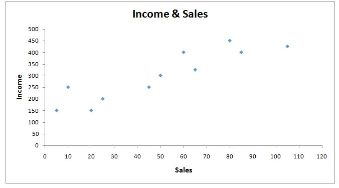
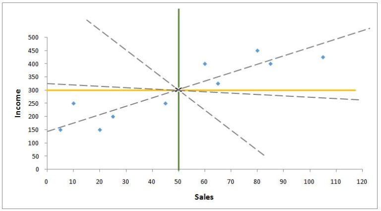
Before getting into detail, let us intuitively understand how regression works. We have a dataset, and a regression line is required to predict the values of Y for a given X. Let us draw some lines on the scatterplot to understand why we need to find the right regression line (good fit).

Several candidate regression lines drawn through the same scatter of data points — Multiple candidate regression lines.

We can see how many regression lines can be created; however, there can be only one line that gives us the best prediction. Here, better prediction means less error, and this is precisely what the Linear Regression Model does when it uses Ordinary Least Square Regression to produce this regression line. The regression line here is the predicted value, while the distance between the data points and the regression line is the error. When we take the square of this distance and sum all these squared distances, the result is known as the Sum of Squares, also known as the Sum of Squared Deviations. The regression line under OLS regression is drawn where the line produces the least amount of sum of squares.

Calculating the Regression Equation / Best Fit Line

There are three ways through which we can understand how this best line is calculated.

Intuitive Way

First is the intuitive way. For example, we use a statistical software, and in the backend the software starts to give slope to this regression line and tries various permutations and combinations with multiple kinds of lines, such as low-slope, negative-slope, etc., and finally comes up with the line where the sum of square error is the minimum. This happens because different lines have a different distance from the actual data points, and the ‘Best Fit Line’ is selected where the sum of squared deviations is the minimum. Through this method, the software is able to provide us with the intercept and the beta value.

Mathematical Way

Second is the Mathematical way. We can use certain statistics to compute the beta coefficient, such as mean, standard deviation, and correlation coefficient. Now we can use a formula to find the beta value (regression coefficient):

b = r × (s_y / s_x)

where,
b is the beta value,
r is the correlation between the X and Y variables,
s_y is the standard deviation of the Y variable,
s_x is the standard deviation of the X variable.

Thus, by using the above formula, we are able to find the value of the beta value:

Worked calculation of the beta coefficient using means, standard deviations and correlation coefficient — b = 0.91 × (108.97 / 32.63) = (0.91) × (3.339) = 3.038

This value (b) is the unstandardized (raw) regression coefficient, expressed in the original units of the variables. It is obtained by taking the correlation coefficient r - which is scale-free - and multiplying it by the ratio of the standard deviations (s_y/s_x), thereby putting it back onto the original scales of measurement. The standardized coefficient is different: in simple linear regression it is simply equal to the correlation coefficient r, and being scale-free it lets us compare the influence of variables measured on different scales. (How correlation relates to simple linear regression is discussed at the end of this article.) The raw coefficient b is also called the unstandardized regression coefficient, while the scale-free version is called the Standardized Coefficient, Beta Coefficient, Beta value, or Beta Weight.

Once we have the beta value, we can calculate the alpha value, which is the y-intercept. This can be calculated by the following formula:

a = Ȳ − bX̄

where Ȳ is the average value of Y, X̄ is the average value of X, and b is the regression coefficient. Thus the formula for our example will be:

a = 300 − (3.038)(50)
a = 300 − 151.9
a = 148.1

The intercept value of 148.1 means that when the value of x is 0, the value of y will be predicted as 148.1.

y = α + βx
y = 148.1 + 3.038 × 0
y = 148.1

However, this can't be true and is a bit unrealistic. This is the reason why an additional component of error is added to the formula. As the simple formula for Y is Y = a + bx (same as y = α + βx and y = mx + c), the formula with the error component can be expressed in two ways:

e = y − ý
or
e = y − (α + βx)

(here α + βx = ý means predicted y). Therefore we can have two regression formulas: one for the predicted value of y, and one for the observed value of y, where the error can be known and considered in the prediction.

Thus we can predict the Y value given a value of X. For example, if a person has sales of 55, then what will their income be? The solution will be:

y = α + βx
y = 148.1 + (3.038)(55)
y = 315

Thus the income for sales of 55 will be 315, plus or minus the error term. Another way of understanding the regression coefficient being 3.038 is that for a unit increase in sales, keeping all other variables the same (for multiple regression), the income will go up by 3.038.

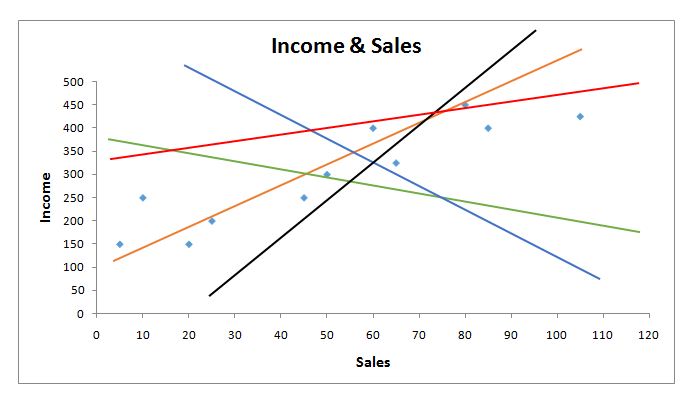
Finding Best Fit Line in Graph

To find the best fit regression line, we first form a graph with the x-axis having the independent variable and the y-axis having the dependent variable. We then find the mean of both these variables on the graph.

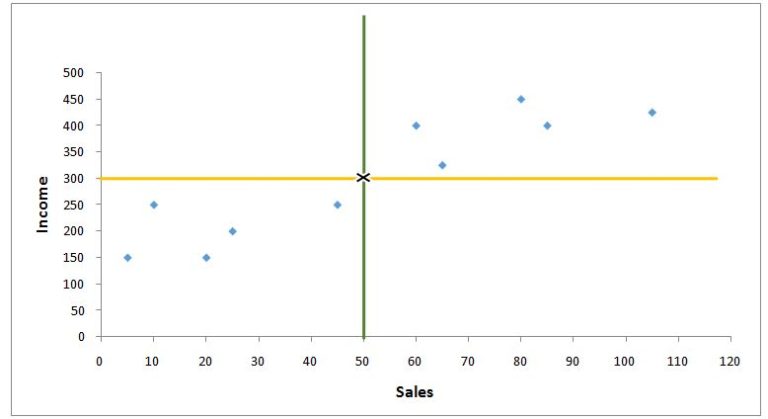
Graph showing the mean of the independent and dependent variables intersecting at a point — The mean of both variables intersects at a single point.

As shown above, the mean of both of these variables intersects at a point (where the mean of both the dependent and independent variable cross), and this is the point through which all regression lines have to pass. Now the question is to find the intercept value, i.e. the point on the y-axis through which the regression line will pass, providing the minimum sum of square error / residual / sum of squares / sum of squared deviations.

Multiple possible lines passing through the mean intersection point — Several possible lines can pass through the intersection.

We can see how several possible lines can pass through the intersection; thus we need to find the point where the line intersects the y-axis. To find the intercept value, the distance from each x value to the mean is calculated for all observations, and the same is done for y, where the distance of each observation from the y mean is calculated.

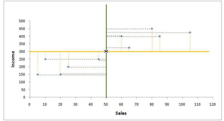
Graph showing distances of each observation from the means of x and y — Distance of each observation from the mean of x and y.

Thus we can have the difference of both variables' values from their respective mean (x − x̄ and y − ȳ). We then square the difference of the independent variable's values from their mean and sum them (∑(x − x̄)²). We also multiply the difference of x values from their mean with the difference of y values from their mean, and sum them (∑(x − x̄)(y − ȳ)).

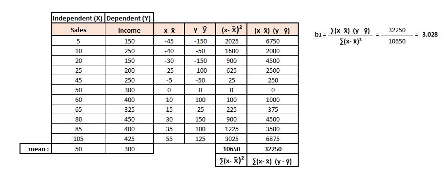
Table of x and y deviations from their means used to compute the regression coefficient — Computing the sums needed for the regression coefficient.

In this section, the terms that will be used are b0 and b1, where b0 (pronounced ‘beta nought’) means intercept and b1 means the beta value. Therefore the equation for the regression line will be ý = b0 + b1x. To find the beta value (i.e. the slope of the regression line), we divide ∑(x − x̄)(y − ȳ) by ∑(x − x̄)², and this gives us b1.

Now we find b0 (the intercept value) by using the available values in the equation. The equation of the regression line is ý = b0 + b1x. Here the ý will be the average of the y variable, while the x will be the average of the x variable. We use these values because a regression line has to pass through these coordinates (50, 300). Thus the equation will be:

300 = b0 + 3.038(50)

We can shuffle this equation to find b0:

300 = b0 + 151.9
300 − 151.9 = b0
148.1 = b0

We can now draw the Best Fit Line by using both points (the intersection of the mean of the x and y variable, and the intercept).

Thus there are multiple ways through which we can find the best regression line. The points that fall on this line are the predicted values for a given value of x.

Simple Linear Regression v/s Correlation

Correlation measures the degree to which two variables are related to each other, but it doesn't distinguish between independent and dependent variable, whereas in Linear Regression there is always an independent and a dependent variable, where the values of the dependent variable are predicted given the values of the independent variable. The output of linear regression, in most statistical software, provides us with information on how the two variables are related to each other. Thus the Correlation Coefficient (r) is equal to the standardized regression coefficient; the raw (unstandardized) regression coefficient b differs from r only by the ratio of the standard deviations (b = r × s_y/s_x). However, running a Linear Regression is more beneficial in some ways, as it can be used to predict the value of the dependent variable. However, there is not much difference between Simple Linear Regression and Correlation, and the real benefit of regression can be availed when using Multiple Linear Regression.

Multiple Linear Regression

Multiple Linear Regression is the same as Simple Linear Regression but has more than one independent variable. For example, if we add another variable, ‘experience’, to the example used above, then we will have two independent variables, ‘sales’ and ‘experience’. Then these two variables will have their own regression coefficient, which will be used to predict the value of the dependent variable. Here, however, a regression ‘line’ won't be constructed; rather, a hyperplane of best fit will be constructed.

The formula for a regression plane (having 2 independent variables) will be:

Y = α + β1x1 + β2x2 + ε

where,
α is the y-intercept,
β1 is the beta value (the regression coefficient) for variable ‘x1’,
x1 is the value of the independent variable ‘x1’,
similarly, β2 is the beta value (the regression coefficient) for variable ‘x2’,
x2 is the value of the independent variable ‘x2’,
ε is an error term / random error / noise,
Y is the dependent variable / Y-variable / response variable whose value will be predicted.

In Simple Linear Regression, we found an error, which meant that we were unable to explain some variance in our dependent variable with one independent variable. Thus there can be other variables, such as a second predictor variable ‘Experience’, to explain the income of a person. Thus, when we combine the sales of a car dealer and the experience he has in business, we may be able to reduce the error by explaining more variation in the income. Thus, to reduce the unexplained variance, i.e. error, we add variables to make our predictions better.

Thus Multiple Linear Regression provides us with beta values for multiple independent variables and, like ANCOVA, tests whether an independent variable is related to the dependent variable after controlling for the other independent variables, and explains how strongly each of the independent variables is related to the dependent variable.

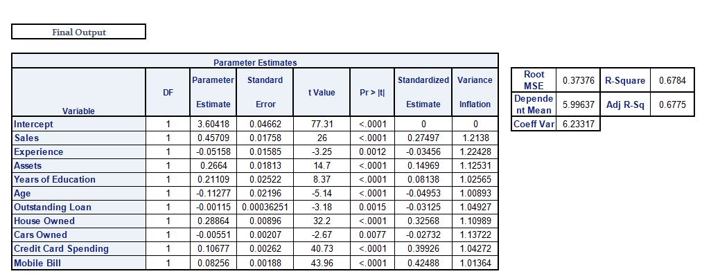
Regression Modeling

Linear Regression, especially Multiple Linear Regression, is used for Regression Modeling, where we are provided with data and have to predict the values of the dependent variable. For example, we have 10 independent variables, and we use all 10 independent variables in a statistical software to create a regression model and get the beta coefficients, intercept, and error term, and use the linear regression equation to predict the value of the dependent variable.

Output table from a multiple linear regression model showing coefficients and significance values — An output from a Multiple Linear Regression Model.

Thus a regression model helps in predicting the dependent variable's value for given values of the independent variables. However, it is important to understand that the process doesn't stop at creating a model. There are various factors that have to be considered, such as the problem of multicollinearity and related concepts such as underfitting and overfitting of the model. To understand this, statistical concepts such as R-square and Adjusted R-square have to be explored. We also have to explore problems such as Heteroscedasticity and Autocorrelation, faced by Linear Regression Models. Thus we need to evaluate our model, and these are explored under Model Evaluation for Regression Models. Also, the eventual purpose of creating a model is to use it against unseen data, and to do this we require validating our model, to be sure that the independent variables that seem important and their corresponding coefficients are those which will provide us with the best result when used to predict values for unseen data (i.e. data the model has not been created on). To do this, various methods have been explored under Model Validation.