// classification problems

Naive Bayes

Naive Bayes is a modeling technique used for solving classification problems where the Y variable can have more than two classes. When the independent variable is categorical, frequencies are used, while for continuous variables, a Gaussian density function is used to compute the probabilities.

Naive Bayes is based on the Bayesian Theorem. Before getting into the details of the theorem and a detailed explanation of the working of Naive Bayes, let's first understand a practical application of Naive Bayes, as it will be very easy to understand the working of Naive Bayes with an example. In this example, we will be only dealing with categorical independent variables.

Quick Example

We have a dataset with 4 categorical variables and a binary dependent variable.

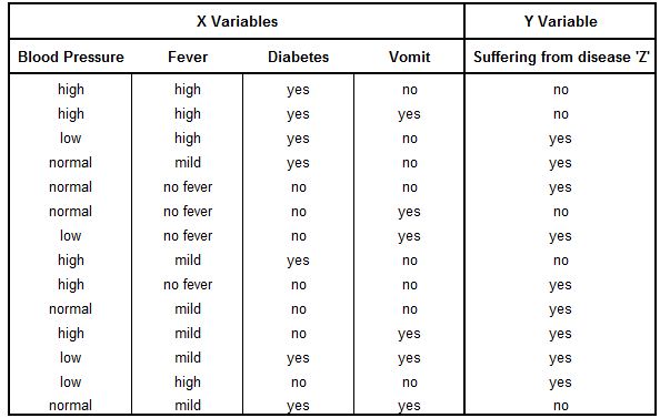
Here we have a dataset where there are 4 X variables that can be termed as symptoms, while the Y variable states whether the person is suffering from a disease ‘Z’ or not. We require Naive Bayes to provide us with a prediction of whether a person who has no fever but suffers from high blood pressure, diabetes, and vomiting is suffering from disease ‘Z’ or not. We can calculate this using the formula below.

P(c|x) = [P(x|c) × P(c)] ÷ P(x)

To come up with the inputs we require, we need to do some calculations.

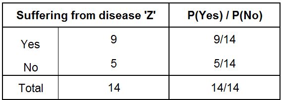
Step 1

Determine how many Yes and No there are in the Y variable. Here we can say that the Probability of the class, P(C), which in our example is a person suffering from disease ‘Z’ or not. Therefore the probability of a person suffering from disease ‘Z’ is 9/14, while the probability of a person not suffering from disease ‘Z’ is 5/14. Here we simply calculated the count of observations from each class of the dependent variable (Yes/No) and divided it by the total number of observations.

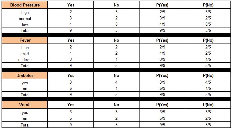
Step 2

Now we calculate individual probabilities for each class of each x feature. Let's take the first feature as an example. We calculate the probability of suffering from disease ‘Z’ for the variable ‘Blood Pressure’ and class ‘high’, which comes out to be 2/9. We also find the probability of a person not suffering from disease ‘Z’ for the variable ‘Blood Pressure’ and class ‘high’, which comes out to be 3/5. We do the same for all the classes of all the x variables and come up with the following table:

Step 3

Now let's consider the question at hand, which is whether a person who has no fever but suffers from high blood pressure, diabetes, and vomiting is suffering from disease ‘Z’ or not.

To find this, we first find the probabilities of a person suffering from disease ‘Z’ for Blood Pressure=high, Fever=no, Diabetes=yes, and Vomit=yes from our table above.

Thus the probability of a person suffering from disease ‘Z’ for blood pressure=high, i.e. P(Blood Pressure = high | Suffering from disease ‘Z’ = yes) = 2/9.

Similarly, we find this for the other variables:

P(Fever = no | Suffering from disease ‘Z’ = yes) = 3/9
P(Diabetes = yes | Suffering from disease ‘Z’ = yes) = 3/9
P(Vomit = yes | Suffering from disease ‘Z’ = yes) = 3/9

We similarly calculate the probability of a person not suffering from disease ‘Z’ for the same set of symptoms and come up with the following probabilities:

P(Blood Pressure = high | Suffering from disease ‘Z’ = no) = 3/5
P(Fever = no | Suffering from disease ‘Z’ = no) = 1/5
P(Diabetes = yes | Suffering from disease ‘Z’ = no) = 4/5
P(Vomit = yes | Suffering from disease ‘Z’ = no) = 3/5

Step 4

We have to multiply all the probabilities for disease ‘Z’ equals ‘yes’ for all the variables (dependent as well as the independent variables). This calculation forms the numerator of the Naive Bayes formula.

For Z = ‘Yes’:

P(X | C) = (2/9) × (3/9) × (3/9) × (3/9) = 0.222 × 0.333 × 0.333 × 0.333 = 0.00823
P(C) = 9/14 = 0.642857
P(X | C) × P(C) = 0.00823 × 0.624857 = 0.005291

We do the same calculation where this time C is the probability of a person not suffering from disease ‘Z’:

P(X | C) = (3/5) × (1/5) × (4/5) × (3/5) = 0.6 × 0.2 × 0.8 × 0.6 = 0.0576
P(C) = 5/14 = 0.357143
P(X | C) × P(C) = 0.0576 × 0.357143 = 0.020571

Step 5

This is the step where we find the denominator of the Naive Bayes formula. Here we divide the above calculations by the probability of X (evidence) to normalize the results.

The value of the probability of X is found by dividing the total cases of a class by the total number of samples. In our example, we are dealing with Blood Pressure=high, Fever=no, Diabetes=yes, and Vomit=yes. In our data we have 5 instances where Blood Pressure was equal to high, similarly 4 for Fever=no, 7 for Diabetes=yes, and 6 for Vomit=yes. We divide each of these values by the total number of samples and then multiply them all together.

P(X) = P(Blood Pressure = high) × P(Fever = no) × P(Diabetes = yes) × P(Vomit = yes)
P(X) = (5/14) × (4/14) × (7/14) × (6/14)
P(X) = 0.357143 × 0.285714 × 0.5 × 0.428571
P(X) = 0.021866

We can also find almost the same value by simply adding the final values found in Step 4: 0.005291 and 0.020571.

Step 6

This is the final step, where we divide both the values found in Step 4 by the value found in Step 5:

P(Suffering from disease ‘Z’ = yes | X) = 0.005291 ÷ 0.021866 = 0.241974
P(Suffering from disease ‘Z’ = no | X) = 0.020571 ÷ 0.021866 = 0.940776

Now we look at both probabilities and find that the probability of not suffering from disease ‘Z’ is greater, and thus we conclude that the person with such symptoms is not suffering from disease ‘Z’.

Understanding the Steps in Context of the Formula

Naive Bayes is a supervised classification algorithm that creates a generative model to solve the classification problem, and its decision boundary is generally non-linear (when visualised, it can be a straight line, but also a circular, elliptical, or parabolic curve). Naive Bayes is a sub-type of a Bayesian Classifier.

Bayesian Classifiers belong to the family of probabilistic classifiers. In this site, we have mainly discussed modeling algorithms whose goal is to learn a function that looks at the input data (x variables) and makes predictions (y variable); however, in a probabilistic classifier, the class is predicted based on the computed probability of that class, so it first computes the probabilities of a class and then the highest probability is picked to come up with a prediction.

Thus, unlike other models where the function looks something like f(x) → y (learn a function from the input x to predict a y), in a probabilistic classifier we compute y = argmax P(c|x) (compute the quantity y, which is P of c given x, for all the classes of c).

In our example, a person has disease ‘Z’ or not, so x will be the various symptoms and c will have two classes: yes (has disease ‘Z’) and no (doesn't have disease ‘Z’). Our classification model will come up with two values: the probability of a person having disease ‘Z’ given those symptoms, and the probability of not suffering from that disease given those symptoms. It then looks for the class with the maximum probability and predicts accordingly. To come up with the probability for each class of c, we have to calculate various other probabilities. In Bayesian-related classifiers we use the following formula:

P(c|x) = [P(x|c) × P(c)] ÷ ∑[P(x|c′) × P(c′)] = [P(x|c) × P(c)] ÷ P(x)

Here P(c|x) means the probability of a person having disease ‘Z’ given a set of symptoms. We find this using a Bayesian formula where the numerator is found by looking at the probability of x given c, multiplied by the probability of c. This is then divided by P(x), which is the sum across all possible classes of c, i.e. the probability of x given a class multiplied by the probability of that class.

Thus we have 3 components to deal with: prior probability, class conditional probability, and the normalizer.

Prior Probability: P(c), the probability of a class of c - in our example, the probability of a person having disease ‘Z’ independent of the symptoms.

Class Conditional Probability: P(x|c), assuming that a person has disease ‘Z’, how likely we are to see a particular symptom occurring or not occurring.

Normalizer: P(x), a normalizing constant.

Prior Probability

In our example, c is whether a person suffers from disease ‘Z’ or not, and P(c) is the prior. What we mean by calculating it is that, without even checking the symptoms of a person (without considering the x variables), what are the chances of a person suffering from disease ‘Z’. Let's assume disease ‘Z’ is very rare; then the probability of suffering from disease ‘Z’ will be very low. Thus, in our dataset of 1000 records, if the number of times the dependent variable is Y=1 (person suffers from disease ‘Z’) is only 10, the class prior probability will be very low. Thus, even if these 10 records have all the symptoms related to disease ‘Z’, the chances of a person having such a disease will remain low. This value helps in providing us with a degree to which we can believe the model is accurately classifying based on the prior data.

Class Conditional Probability

This is x given a class of c - say, for a person having disease ‘Z’, how plausible is the set of symptoms we are seeing related to disease ‘Z’. So, for example, if he has high fever, assuming he has disease ‘Z’, how likely is that. This is computed to find how well the model predicts.

Normalizer

The normalizer is P(x), the denominator, and is often left out of the calculation of the Bayesian classifier, as it doesn't affect the classification. To understand this mathematically, the Bayesian formula for both classes of c will look like:

P(c=1|x) = P(x|c=1) × P(c=1) ÷ P(x)
P(c=0|x) = P(x|c=0) × P(c=0) ÷ P(x)

When we compare the above two equations, we can cancel out the P(x) term, as it is the same for both classes. We are then left only with the numerator, and that is enough to predict the class of a given input. Therefore we can ignore the probability of the set of symptoms unconnected to any class (in our example, the probability of a person having high fever, regardless of whether the person is suffering from disease ‘Z’ or not). As this value is the same for both classes, it doesn't affect the maximum probabilities for the classes of c, and can be ignored. Thus the answer for our example was found in Step 4 alone.

Using all 3 of these components, we are able to come up with the posterior probability P(c|x), whose value means the degree to which we believe the model has accurately classified, given the input and prior information.

Calculation for Continuous Variables

In our example, if the independent variables Blood Pressure and Fever were continuous, the calculation would have been a bit different. We would have calculated the mean and standard deviation of these continuous variables for each class of the dependent variable. Say we find that the mean of Blood Pressure when Y=1 is 73, while it is 75 when Y=0. Similarly, we find that the standard deviation of Blood Pressure when Y=1 is 6.2, while it is 7.90 when Y=0. We do the same for Fever and come up with two values for the mean (79 when Y=1 and 86 when Y=0) and standard deviation (10.2 when Y=1 and 9.7 when Y=0).

Coming back to the formula, we focus on the numerator, where P(c) remains the same; however, the calculation for the Class Conditional Probability, P(x|c), differs, as the probability for a given x is found in a different manner for a continuous variable. We use a probability density function that looks like:

f(x) = [1 ÷ (σ√(2π))] × e^{−(x−μ)² ÷ 2σ²}

Now, for a value of Blood Pressure being 66, what will its class probability be for the class ‘person suffers from disease ‘Z’’? We use the probability density function above and come up with a value of 0.0340:

f(Blood Pressure = 66 | Suffering from disease ‘Z’ = yes) = [1 ÷ (6.2 × √(2π))] × e^{−(66−73)² ÷ (2×6.2²)} = 0.0340

We have to do this for both classes of c, for all the continuous variables, for given values of the x variables. We now use these values to find the numerator of the formula:

When C = person is suffering from disease ‘Z’:

P(X | C) = (0.0340) × (0.2221) × (3/9) × (3/9) = 0.0340 × 0.2221 × 0.333 × 0.333 = 0.008374
P(C) = 9/14 = 0.642857
P(X | C) × P(C) = 0.008374 × 0.624857 = 0.005232

We do the same calculation where this time C is the probability of a person not suffering from disease ‘Z’:

P(X | C) = (0.0291) × (0.0380) × (4/5) × (3/5) = 0.0291 × 0.0380 × 0.8 × 0.6 = 0.000531
P(C) = 5/14 = 0.357143
P(X | C) × P(C) = 0.000531 × 0.357143 = 0.00019

We can now normalize these by dividing by the normalizer value, which here will be 0.005232 + 0.00019 = 0.005422.

Thus the probability of a person having disease ‘Z’ comes out to be 0.005232 ÷ 0.005422 = 0.964958, while the probability of a person not having disease ‘Z’ comes out to be 0.00019 ÷ 0.005422 = 0.035042. As the probability of suffering from disease ‘Z’ is higher, we conclude that the person is suffering from disease ‘Z’.

Limitations of Naive Bayes

What separates Naive Bayes from any other Bayesian Classifier is the naive assumption that the x variables are independent of each other. However, it is generally seen that Naive Bayes works even when the x variables are not independent of each other; the violation of the assumption may simply cause the predictions to be less accurate. As the Naive Bayes theorem gives equal importance to all the variables, it is important to ensure there is no multicollinearity among the variables, and that redundant and identical variables are not used in the calculation.

For numerical variables, it assumes they have a normal distribution, as the probability density function (used in the Bayes theorem when the independent variables are continuous) requires numerical variables to be normally distributed for it to function properly.

Also, if a class of a categorical variable is missing in the training dataset and comes up in the test dataset, the Naive Bayes model will fail to come up with accurate predictions, because the class-conditional probability will be equal to zero. To counter this ‘zero frequency’ problem, various smoothing techniques are used, such as Laplace Estimation, where we add 1 as an additional smoothing term so that the algorithm doesn't divide by 0.

Also, Naive Bayes is sensitive to outliers, so outlier treatment is a must when running such a model. Also, if using Naive Bayes for text classification (spam vs. not spam, etc.), the model can break when it tries to classify phrases - as when Google implemented it and people searched for the term ‘Chicago Bulls’, the output came back with images of bulls and the city of Chicago, rather than images of the American basketball team, the Chicago Bulls.

Advantages of Naive Bayes

Naive Bayes is very easy to implement and is a fast, high-performance method that is able to solve many real-life classification problems and performs fairly well in multiclass classification problems. It also requires less training data than logistic regression may require, and creates a very robust model when there are a lot of features (as many as 2,000 features and more), which is the reason it is popularly used for spam detection and other problems where words form features, making the dataset very high-dimensional.

Naive Bayes is a very effective method for classification problems and has its own set of advantages and disadvantages. It updates the probabilities as more and more evidence becomes available, and thus works well with a good amount of data. It is always a good idea to compare the accuracy of Naive Bayes against other more sophisticated classification algorithms such as SVM and ANN, as it has been seen that the accuracy of Naive Bayes often comes at par with the accuracy of these sophisticated and far more complicated algorithms. Thus, using Naive Bayes is a good idea when dealing with a classification problem.