// shared: regression & classification

KNN - Alternatives to Majority Voting

In K Nearest Neighbour, majority voting is used to pick the class for prediction. However, this method suffers from a drawback: if a class is very frequent in the data, then it can hijack the majority voting process and cause the results to be skewed. Therefore a kind of weighted voting may be required to counter such a problem. To understand how the alternative to majority voting works, we need to understand certain concepts such as Parzen Windows and Kernels.

Parzen Windows

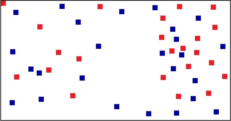
To understand how Parzen Windows work, let’s compare how different it is from the standard KNN method. For example, we have a dataset with two classes, 0 and 1. Below is the 2-D representation of the data points, where 0 is represented by a Blue Square and 1 is represented by a Red Square.

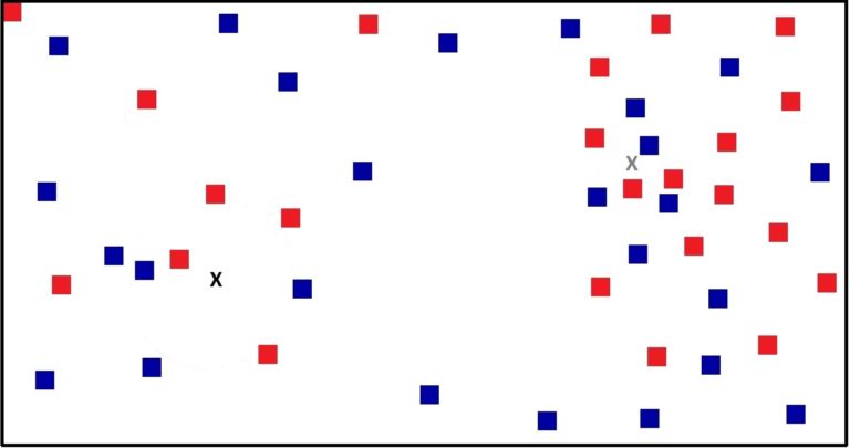
2D scatter plot of data points belonging to two classes, with class 0 shown as blue squares and class 1 shown as red squares

Now let’s take two different points that we need to predict. These two testing points are represented as X (in black colour) and X (in grey colour) in the figure below.

The same scatter plot with two unlabelled testing points marked, one in black on the left cluster and one in grey on the right cluster

Now if we apply KNN with the value of K being 5, then for the Black X point, it finds the 5 nearest data points, and these 5 data points together form a radius under which all 5 data points lie. We can say that the KNN algorithm will predict the data point on the basis of this radius under which these 5 data points lie. Similarly, for the Grey X point, the 5-NN algorithm finds the five closest data points, and these data points all lie under a radius as well. However, if you notice, the radius of the Black X point is much larger than that of the Grey X point.

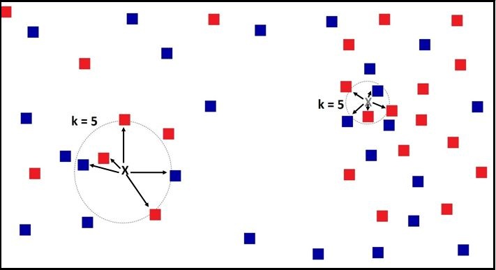
Two clusters each with a circle drawn around their five nearest neighbours to a testing point X, where the circle on the sparser left cluster has a much larger radius than the circle on the denser right cluster, both for k=5

This is because the data points on the left are very scattered, and for a testing point placed here, we have to look far away to come up with 5 data points, whereas on the right side the data points are dense, and therefore the radius here is much smaller.

We can now understand how the Parzen Window algorithm is different. While KNN looks for a fixed number of data points/neighbours, Parzen Windows look for a fixed area of the region to find the data points that are included to predict the unknown data point. Therefore in Parzen Windows, the radius remains the same, while the number of data points varies.

To understand this intuitively: if you are asked to collect samples from your neighbourhood about the number of members in a house, then the criteria for deciding the number of samples can either be the number of houses - e.g. the 5 closest houses from your home - or it can be a region, i.e. all the houses 200 metres from your home, and if you live in a dense city like Mumbai, then you may end up with a lot of samples if you choose the latter method.

Below we apply the Parzen Window method to both testing data points, where the radius R is fixed.

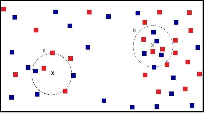
The same two clusters, now each with a circle of identical fixed radius R drawn around the testing point, where the sparser left cluster's circle captures fewer points than the denser right cluster's circle

We can see that this time, for the Grey X point we have 9 data points to decide from, while previously we had only 5. Similarly, when we look for the region of radius R for the Black X point, we get roughly the same number of data points as when we used 5-NN, as the radius of both is almost the same. Thus the idea of neighbourhood exists in both methods; however, in KNN the neighbourhood has a fixed number of data points, while in Parzen Windows the neighbourhood has a fixed area.

The equation for Parzen Windows looks like this:

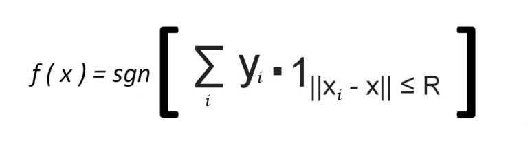
Formula: f(x) equals sgn of the sum over i of y sub i times the indicator function 1 when the norm of x sub i minus x is less than or equal to R

Here, for example, for every red point a label of +1 is assigned, and for blue a label of −1 is assigned. Now we decide the neighbourhood around a test data point (e.g. the Grey X) based on the radius R, and come up with a certain number of data points whose labels are added up. Thus if we get a negative value in the end, we predict the point to be a Blue Square, which is what we get for the Grey X testing point.

Thus we decide the class of the data point on the basis of the sign of the sum of the labels. The above equation can be understood as follows: we first go over all the training data points, and with the help of an indicator function - which is 1 when a data point is inside the radius R and 0 when it is outside - we are able to identify the data points to be considered. Therefore, when the distance between the unknown testing point (x) and a training data point (x_i) is less than or equal to the predetermined radius R, the class label of that data point is considered.

Note that this algorithm only works for Binomial/Binary classification.

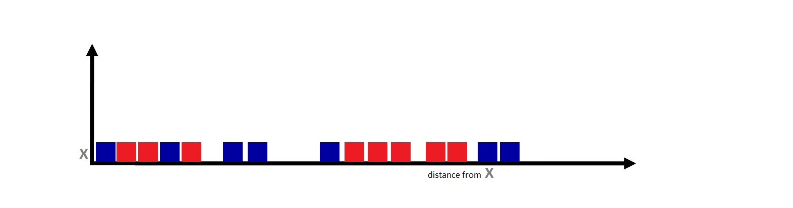
Below is a graph plotting the Euclidean Distance of data points from the Grey X testing point along an axis.

A number line labelled distance from X, with the data points nearest to X plotted at increasing distances along the axis, coloured by class

Now if we apply the Parzen Window, where the indicator function uses a value of R (radius) that divides the data between considerable and non-considerable, we get the following figure:

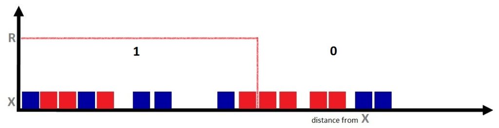
The same number line with a cutoff marked at radius R, where all points within R are labelled 1 (considered) and all points beyond R are labelled 0 (not considered)

Here we can see that all the data points within the radius get a value of 1, i.e. they are considered, while the data points outside the radius R are deemed inconsiderable. Therefore, according to the Parzen Window algorithm, the Grey X point will be predicted as a Blue Square. However, we are still using majority voting only, and we require a more sophisticated method - which brings us to an extension of Parzen Windows: the Kernel Function.

Kernels

If you analyse the above figure closely, you’ll realise that we suffer from a major drawback in assigning the class label. In the figure above, right after the radius cutoff we have two red data points, and the value of their class labels is completely ignored because they weren’t able to make it inside the radius, even though the difference in distance is minute. If we increase the value of R, we’ll be able to include those two red points, which would completely change our prediction, and the Grey X point would instead be predicted as Red. And if we increase the value of R only slightly, we may end up with 5 blue and 5 red, thus running into the issue of ties.

Therefore our algorithm is very sensitive to the value of R, and the value of R can greatly shift the prediction - which is fine during the training phase, but can create problems during the model testing/validation phase, as we might be unable to generalise the model well enough to make good predictions on unknown data. Thus we can come up with a kernel function, where we get a much smoother function instead of the box-shaped Parzen Window function, where the values of the data points are not a fully considerable 1 and then suddenly a fully unconsiderable 0.

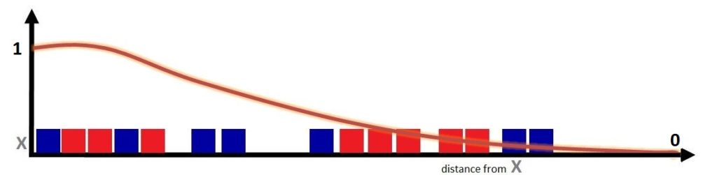
The same number line, now with a smooth decaying curve overlaid instead of the hard 1/0 cutoff, starting near 1 close to X and gradually decaying toward 0 as distance increases

In a Kernel, we don’t assign weights as a hard 0 or 1, but instead distribute the weights such that they are proportional to the inverse of the distance from the unknown point to the test data point, so the data point closest to the unknown point contributes more, while the contribution of the data points diminishes as they move farther away from the unknown data point. Thus this gradual decay allows data points at close distances to have weights around 1, with a continuous decrease in this value as the distance increases.

The Kernel function helps transform smaller distances into higher weights and vice versa, and ends up providing us with weighted voting. Thus we are able to control the effect of the variance introduced by K in KNN and by R in Parzen Windows.

The equation for this decaying kernel function looks like this:

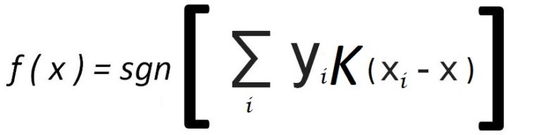
Formula: f(x) equals sgn of the sum over i of y sub i times K of (x sub i minus x), where K is the kernel function

If we compare the Parzen Windows equation with the equation above, we can see that we simply replace the indicator function with a kernel function between the testing point x and training point x_i, where K is based on the distance between x and x_i and decays from a large value to a small value.

Thus we can use the Kernel function to provide us with a more robust, generalised model that assigns weights to the data points - a better method than plain majority voting.

The alternatives to majority voting discussed above help make the model more stable and increase its accuracy. While Parzen Windows and the Kernel function both help provide a more unbiased estimate, the Kernel function is more effective in providing balanced results than Parzen Windows.