// shared: regression & classification
K Nearest Neighbour
K Nearest Neighbour, commonly known as KNN, is an instance-based learning algorithm, and unlike linear or logistic regression where mathematical equations are used to predict the values, KNN is based on instances and doesn’t have a mathematical equation. As there is no mathematical equation, it doesn’t have to presume anything, such as the distribution of the data being normal, etc., and thus is a non-parametric way of predicting. It is a supervised non-linear method used to solve classification as well as regression problems.
Idea Behind KNN
Let us understand KNN with an example. Suppose we have a dataset where the Y variable has two classes - Squares and Rounds. There is an additional unknown point (black triangle) and we want to know which class it belongs to.
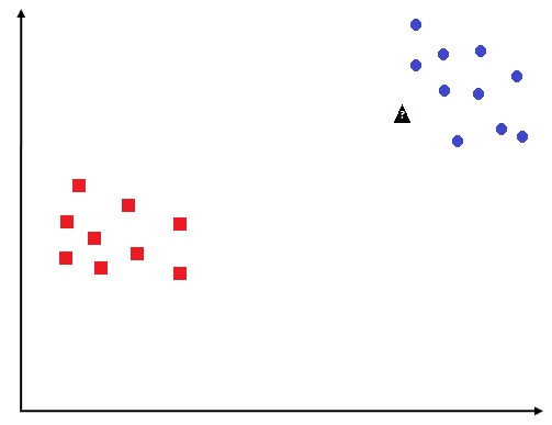
If the same dataset is shown to a child, then unlike computing a prior as done by Naive Bayes, a hyperplane as done by logistic regression, or computing information gain as done by decision trees, the child will simply look at the points that are close to the unknown point and will predict the point to be of that class. This is something that KNN does, where it classifies a data point based on its proximity to the training examples.
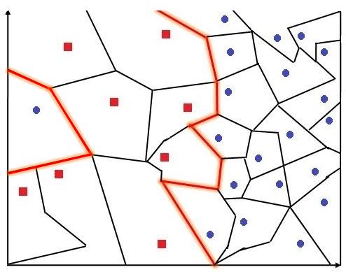
Voronoi cell
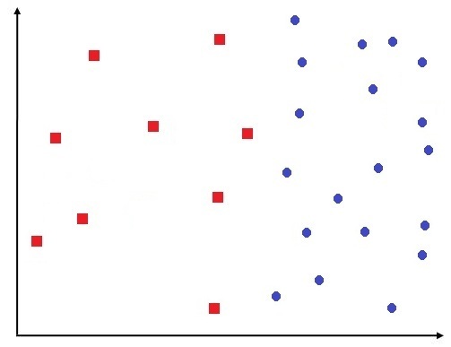
If we have a dataset that looks something like shown below, where the data points of different classes are in more proximity than what was shown earlier.
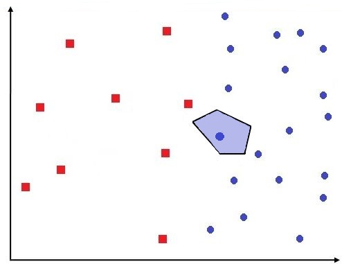
If we set k=1 for our K’s nearest neighbour algorithm, then for each new data point, the nearest training example is found and its class is considered for prediction. To understand this properly we have to first understand what Voronoi cells mean. See below how a blue data point has a region around it, designated as blue, so any point that lies in that area/neighbourhood will be classified as blue. Thus an entire cell is coloured ‘blue’ on the basis of one data point. This blue region forms a Voronoi cell.
Role of the value of K
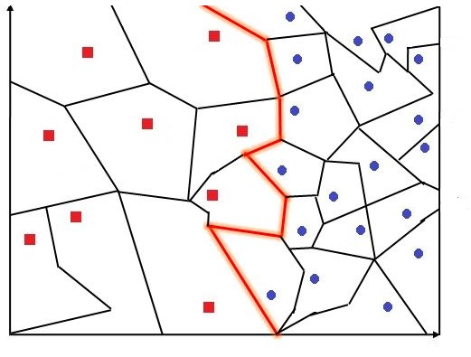
In K’s nearest neighbour, each of these data points will have their Voronoi cell, which is collectively called Voronoi Tesselation. We now can come up with a decision boundary which passes in such a way that it differentiates one class of data points from the other. However, K’s nearest neighbour, even being a very simple algorithm, comes up with a decision boundary that is more complex than what Naive Bayes and Logistic Regression come up with, and is almost at par with decision trees.
To understand why we use k=n and don’t just stick with k=1 for prediction, we have to first go through some of the limitations of KNN, which is that it is very sensitive to outliers and noise, as it can end up shifting the decision boundary very dramatically. For example, if we have a blue data point on the extreme left which is there due to noise/outlier, then the decision boundary will shift drastically, and the whole area around that data point will be labelled as blue while it is clearly in a region dominated by red data points.
Also, unlike Naive Bayes, it doesn’t take into account the prominence of a class and doesn’t have any parallel to a ‘prior’ to see the frequency of one class compared to another. Thus it generates no confidence value. However, if there are data points belonging to a particular class which are overwhelmingly in dominance, then it will affect the majority voting, and to counter this, the value of k has to be tweaked, whereby increasing the number of k we are able to add more stability to our model.
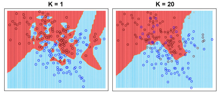
Thus we now look at the way the value of k affects the whole game of KNN. As k=1 will make the decision boundary very sensitive to noise and will end up making the model very complex and unstable. Any small change in the training data will greatly alter the decision boundary.
We can increase the number of k, for example, to 20. Now what we mean by k=20 is that for a given unknown data point, it will look at more than 1 nearest neighbour, i.e. now it will look at 20 neighbours to predict its class. Here the dominant class will be considered for prediction, while the methods of considering a class as dominant can vary and will be discussed further.
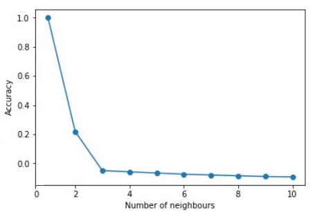
Increasing k, as discussed earlier, will make the model less complex; however, if we take a large enough value of k, say k = no. of samples, then it will simply classify on the basis of the class that occurs most commonly, converting the model into a prior classifier. Thus a large value of k will make the model underfit. To find the right value of k we use grid search along with resampling measures such as cross-validation.
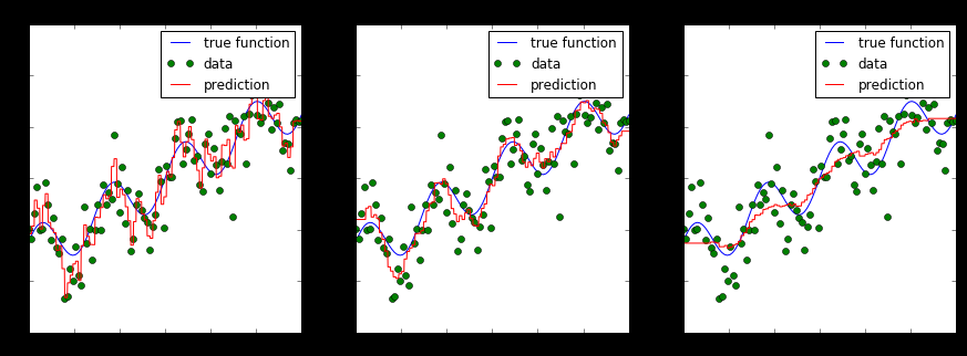
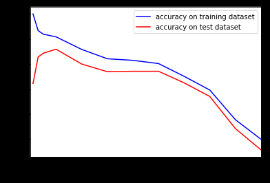
If we take a look at the figure below, we can see how, with a lower value of k, the model becomes a victim of overfitting and is very complex to effectively generalise, while increasing the k smoothens the decision boundary and makes the model more stable.
Working of KNN for a Classification Problem v/s Regression Problem
Classification Problem
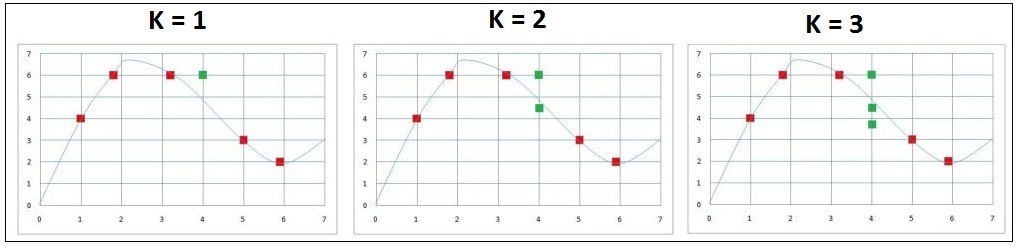
We have the below data with two classes - Red and Green - and we have to find the class of the Yellow Box.
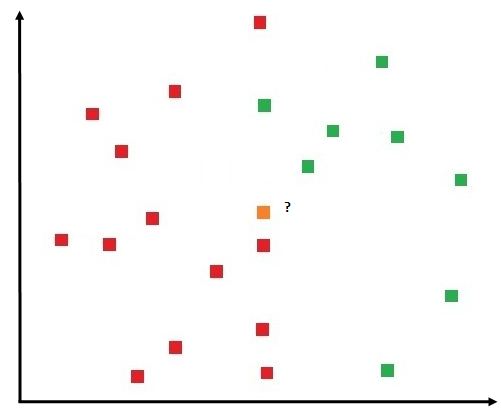
In a classification problem, we take the point that we want to classify and start computing the distance from the unknown data point to every other data point of the training dataset. Now we pick k number of data points that are closest to the unknown data point, and based on the most frequent class, assign the label to the unknown data point. Thus here we use a majority voting system to decide the class of the data point.
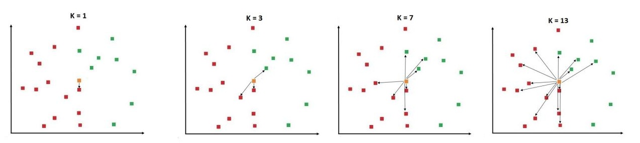
We can see in the above figure that when k was equal to 1, the nearest data point to the yellow square was red, and thus it would have been labelled as a red data point. Similarly, when we increased the value of k to 3, then it got the 3 data points nearest to it, out of which 2 were red and 1 was green. When k was 7, we got 4 red and 3 green, while for k=13 we had 9 red and 4 green data points.
Regression Problem
If the labels that are to be predicted are continuous, then KNN Regression is used.
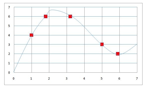
Here also we take the unknown point and compute distances to all the data points and find k nearest data points, and this time, rather than taking a majority vote, we average the value of the Y variable that the nearest data points denote, thus computing the mean of the labels of the k nearest neighbours, and this mean is used as the prediction. Above, we have the 1-dimensional representation of a regression problem, and we have to predict the true function, which is unknown to us. We now try to predict this function from the observations we have.
On the x-axis, we have the values that we want to predict, and on the Y axis we have the various numbers of the Y variable. Now for a given input of 4, if we have to predict the Y, then we look on the x-axis at the point nearest to it (we don’t look at the y-axis, as it represents the Y variable, which is not the basis for prediction; we are predicting Y on the basis of a value of x). We find that the nearest point to 4 is at 3.2, so if we are using k=1 in the algorithm, then this point will be considered and its corresponding Y label will be used to predict the value. Thus for a given value of 4, the Y will be predicted as 6.
However, if we use k=2 in the algorithm, then we consider the two closest values of x, which are 3.2 and 5, and we take an average of their corresponding Y variable, which comes out to be 4.5 ((6 + 3) ÷ 2 = 4.5). Thus for a value of x=4 with k=2, the value of Y will be 4.5. We can do the same with various values of k and settle with the value of k that gives us the prediction which is closest to the true function.
We can see that k=2 gives us the best result. Thus we can see that finding the right value of k is very important, as with a very low value of k, the model becomes complex. On the other hand, a very high value of k, say where k = total number of samples, then the output will be the arithmetic mean of the Y variables.
As mentioned earlier, we can use grid search to test various values of k and find the k that provides the best accuracy.
Methods of Improvement
Till now we have only discussed the value of k as a hyper-parameter that can be tweaked to give us better results. However, there is a lot of scope when dealing with KNN, as there are many parameters and other methods of improvement that can be used to provide us with better results. Some of these methods are: using different distance metrics, alternatives to majority voting, techniques to approximate nearest neighbour, resolving ties, rescaling data, missing value and outlier treatment, and dimensionality reduction.
Distance Metrics
Depending upon the type of features KNN is working with, adjusting the methods of calculating the distance can greatly improve the results produced by KNN. There are various distance metrics other than the usual Euclidean Distance used so far, such as Hamming Distance, Minkowski Distance, etc. You can refer to the blog on KNN Distance Metrics for more information.
Alternatives to Majority Voting
So far the method of voting was majority voting; however, this method can have its own set of drawbacks, because of which other alternatives to majority voting can be used, which can help in improving the results produced by the algorithm. For more information, refer to KNN Alternatives to Majority Voting.
Techniques to Approximate Nearest Neighbour
One of the biggest drawbacks of KNN is that it is very slow in the testing phase, which limits its usage. The main reason for this is that it considers all of the data points when approximating the nearest neighbours, which makes the whole process very slow. There are methods such as K-D Trees, LSH, and Inverted List that can be used to make the whole process faster without losing much accuracy and reducing reliability, and have been explored in KNN - Techniques to Approximate Nearest Neighbours.
Resolving Ties
If we have the same number of votes for different classes, then it becomes difficult to select one class for predicting the unknown data point. When the classes are binary, then an even value of k should be avoided, as an even value of k can lead to ties. So values of k should be odd (1, 3, 5, 7, 9 . . .). However, this technique cannot work with a multiple class problem, and for such cases, we should avoid the value of k from being a multiple of the number of classes. In the event of ties, we can either set the value of k to 1 or can pick a class randomly. A more robust way will be to use a prior, where the class that has an overall high frequency is considered for prediction.
Rescaling Data
Data, when being used for a distance-based model, must be rescaled. For example, we have two features: height of the person in metres and weight of a person in pounds. Here, as the absolute value of weight will be more, the distance metric will be skewed. Therefore, various rescaling methods should be used to rescale the features before using them for KNN. To know about the different scaling methods, refer to Feature Scaling.
Missing Value and Outlier Treatment
Missing and extreme values are very problematic for KNN. All the models that use distance metrics can get negatively affected by outliers, and therefore outlier treatment must be done on the data before using it for a KNN model. Similarly, missing value treatment must be done on the data so that KNN can be performed properly. Refer to Missing Value Treatment and Outlier Treatment for more information.
Dimensionality Reduction
If there are a lot of unnecessary variables (causing multicollinearity), then, unlike decision trees, where it ignores such variables and doesn’t get affected, KNN gets negatively affected, as it gives equal importance to each feature. Thus if the data is in very high dimensions, then KNN doesn’t work properly; therefore, feature reduction methods must be applied to make the distance metric more meaningful and the model more robust.
Pros and Cons
Like all the other algorithms, KNN has its own advantages and limitations.
Pros
It requires no assumption, i.e. it is a non-parametric method, thus we don’t fit any distribution. It can be used for regression as well as for binary and multiclass classification problems. The time taken by KNN in the training phase is much lesser when compared to other models, and is much faster for generating such complex results. And, obviously, it is very easy to understand and is simple to implement.
Cons
It doesn’t work properly if the data has missing values, outliers, too many useless features, or if it is not scaled. Also, the biggest problem of KNN is that, unlike ANN, which is slow at training and fast at testing, KNN is relatively fast at the training phase when compared to the testing phase, where it is extremely slow. This happens because, unlike other models where some function is learnt and is then applied to the testing set, KNN memorises all the instances of the training set. All these instances can be expressed as n. In the testing phase, then, each of these testing samples is compared with n. Thus this makes the process very computationally intensive. Also, as the size of the training data becomes larger, the training phase becomes slower. If using majority voting, then the results can become skewed, as the classes that are frequent in the data will dominate the majority voting process. Thus other methods, such as weighted voting, may be required.
K Nearest Neighbour is a very simple and powerful technique that provides us with a lot of options to generalise our model. It can be used for Classification as well as Regression problems. It faces the problem of being vulnerable to overfitting and being slow; however, there are various methods to go around it. All the hyperparameters discussed in this article must be played with to come up with a KNN model that suits your data and yields good results.