// shared: regression & classification

KNN - Distance Metrics

In KNN, there are a few hyperparameters that need to be tuned to get an optimal result. Among the various hyperparameters that can be tuned to make the KNN algorithm more effective and reliable, the distance metric is one of the important ones, through which we calculate the distance between data points, as for some applications certain distance metrics are more effective. There are many kinds of distance functions that can be used in KNN, such as Euclidean Distance, Hamming Distance, Minkowski Distance, Kullback-Leibler (KL) Divergence, BM25, etc.

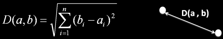
Euclidean Distance

This is among the most common distance metrics used for calculating the distance between numeric data points. The formula for Euclidean distance is as follows:

Let’s understand the calculation with an example. Suppose we have a data point with coordinates (5,2) and a class label of 1, and another point at position (1,5) with a class label of 2.

The distance is calculated as follows:

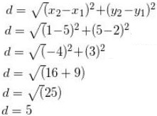
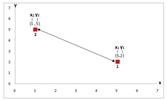
Worked calculation: d equals the square root of (1 minus 5) squared plus (5 minus 2) squared, equals the square root of 16 plus 9, equals the square root of 25, equals 5

Scatter plot of the two points at (5,2) and (1,5), with an arrow showing the distance between them

Thus here the distance is calculated as 5.

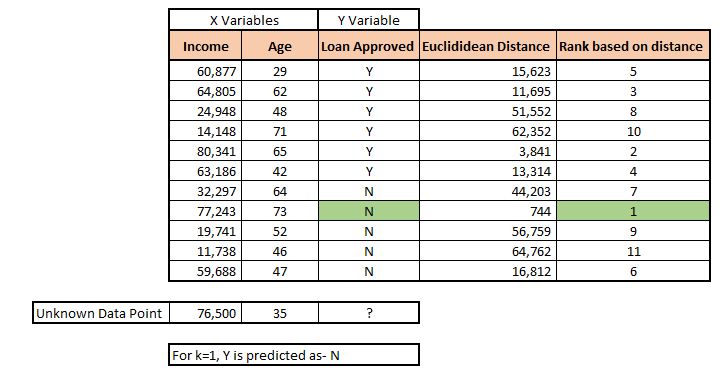
Another way of understanding this is in terms of a dataset. Suppose we have data with two x variables and a y variable. These two x variables are Income and Age. The values of these two variables will act as x₁ and y₁ in our Euclidean formula. Now for a person who has an income of 76,500 and an age of 35, these two values will act as x₂ and y₂. We can calculate the distance, and if we consider k=1, we can assign the class label of the closest data point.

Table of ten data points with Income and Age as X variables and Loan Approved as the Y variable, each with a computed Euclidean Distance and rank, with the closest point at rank 1 having a distance of 744 and Loan Approved equal to N, used to predict the unknown data point's class

Hamming Distance

This distance metric is used when dealing with categorical data. For a given data point, we look at whether its value is equal to the value of the data point against which the distance is being measured. If the two values are the same, we take a 0; otherwise, we take a 1. We then add up the number of differences to come up with the value of the distance. The formula for Hamming distance is:

D(x,y) = Σ_d 1_{x_d≠y_d}

An easy way of understanding Hamming distance is to suppose we have two data points, where the first is represented by the bits 0011 while the second is represented by 1110. This method looks at each bit and compares it with its corresponding bit to see if they match or not.

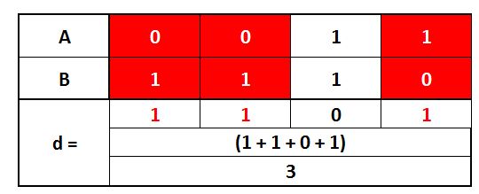
Table comparing bits 0 0 1 1 of point A against bits 1 1 1 0 of point B, with mismatches highlighted in red at the first, second, and fourth positions, giving d equals 1 plus 1 plus 0 plus 1 over 3

We can see that at 3 instances the bits don’t match. Thus the Hamming distance comes out to be 3.

Minkowski Distance

Euclidean distance can be generalised using the Minkowski norm, also known as the p-norm. The formula for Minkowski distance is:

D(x,y) = ^p√(Σ_d |x_d - y_d|^p)

Here we can see that the formula differs from the formula for Euclidean distance, as instead of squaring the difference, we raise the difference to the power of p and also take the p^th root of the result. The biggest advantage of using such a distance metric is that we can change the value of p to get different types of distance metrics.

p = 2

If we take the value of p as 2, we get the Euclidean distance discussed above.

p = 1

If we set p to 1, we get a distance function known as the Manhattan distance.

p = ∞

If we set p to a very high number, the formula behaves like a max function. Thus if we have two values, −4 and 3, then rather than adding them up and taking a square root as done in Euclidean distance, we take the maximum absolute difference as the distance - here we would take 4 as the distance (the larger of |−4| and |3|). We can see that Euclidean distance gave us a value of d=5, while by setting the value of p to infinity, we get d=4. As the value of p is very high, it makes the largest difference dominate the others.

p = 0

We get a function that behaves like a logical AND.

For every value of p, the distance between two data points is measured differently. Thus each of these values is useful in certain conditions. We can use any arbitrary value of p and see which gives us the best results.

Other Specific Methods

Kullback-Leibler (KL) Divergence

This distance metric is used when working with histograms.

BM25

This is a custom distance metric used especially for text-related problems. There are many other custom distance metrics that are very domain-oriented and give the best results when used for a certain kind of problem.

Distance metrics play an important part in the KNN algorithm, as the data points considered in the neighbourhood depend on the kind of distance metric being used. It therefore becomes important to make an informed decision when choosing the distance metric, as the right metric can be the difference between a failed and a successful model.