// shared: regression & classification

KNN - Techniques to Approximate Nearest Neighbours

One of the biggest problems with KNN is the time the algorithm takes during the testing phase. There are various ways to solve this problem, and that is what we’ll explore here.

Reason for KNN Being Slow

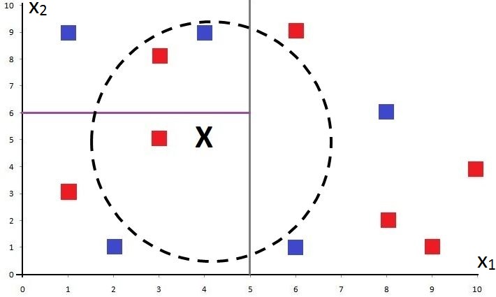
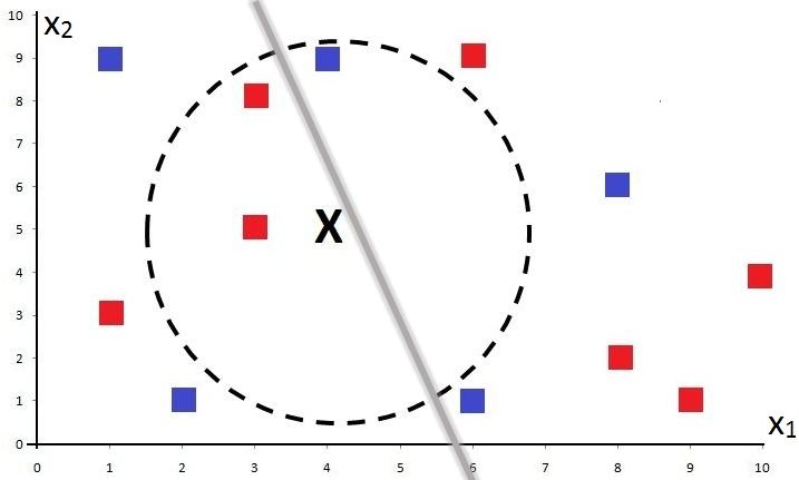
Suppose we have a dataset with 2 features. A 2-D representation of such data, with a missing point to classify, would look something like this:

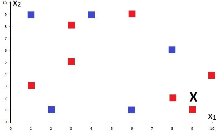
2D scatter plot of blue and red square data points across a grid from 0 to 10 on both axes, with an unknown point X near (9,2)

Just by looking at it, we humans can guess that the unknown point X should probably be classified as a Red Square.

However, the algorithm will read the training points something like this: (10,4), (4,9), (9,1), (1,9), (6,9), (3,5), (6,1), (1,3), (2,1), (3,8), (8,6), (8,2), and the unknown testing point X as (9,2).

Now if we look at the coordinates, we can understand why it might be difficult for the algorithm to find the right classification. The algorithm has to compare the testing point with all the training points, come up with distances, and then, based on the K value, find the K nearest neighbours and come up with a result on the basis of voting.

However, this process becomes very time-consuming if the number of training instances and unknown points is large. If we have N training points and D features, then the testing operation will take N × D time.

To counter this problem, we have two options. We can reduce the number of features to reduce D, or we can reduce N by reducing the number of training points that a testing point has to be compared with in order to come up with K nearest neighbours. This reduced number of candidate points gives us M potential neighbours, which makes the operation M × D - faster than the N × D operation. However, we can only hope that M is greater than our determined K.

Therefore, if we want K=5, then M should be greater than 5 to get any meaningful results. If the sample size is large enough and the value of K is optimal, then M should be a lot more than K. Also, M should be a lot less than N, so we get a considerable reduction in the time taken by the algorithm. There are multiple ways to arrive at M, such as K-D Trees, Locality-Sensitive Hashing, and Inverted Lists.

K-D Trees

We use this method to find potential neighbours when the data has a limited number of continuous features. This method is not effective if the features are sparse, i.e. have a lot of 0s in the data - which is generally the case with categorical features, since creating dummy variables/one-hot-encoding leaves us with a lot of 0s. To understand this method, let’s take the sample data discussed above.

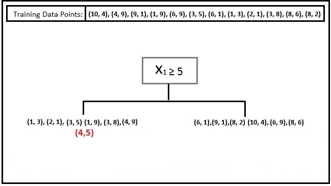
We have a dataset with 2 features, X₁ and X₂, with two classes of data: Blue Squares and Red Squares, with coordinates (10,4), (4,9), (9,1), (1,9), (6,9), (3,5), (6,1), (1,3), (2,1), (3,8), (8,6), (8,2). Thus we have 12 training data points. K-D Trees organise this dataset into a tree, where the unknown testing data point is placed on a leaf of the tree containing the M potential training data points to be used for classifying it.

Let’s say we have a testing point (4,5).

The 12 training points plotted on a grid, with a dashed circle around the testing point X at (4,5) enclosing its 5 nearest neighbours

The K-D Tree algorithm will now take a feature - for example, X₁ - and find its median to split the data such that half of the data lies on one side and half on the other. In our case, let’s say the algorithm picks the value 5 on the x-axis; the data is then divided so that 6 points lie on one side and 6 on the other.

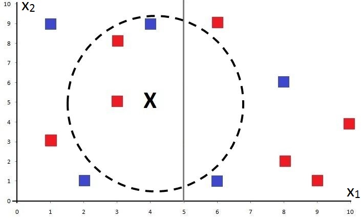
The same plot with a vertical grey line drawn at X1 equals 5, dividing the 12 points into two groups of 6

A tree diagram showing the root node X1 greater than or equal to 5, splitting the 12 training points into a left branch of 6 points (including the testing point 4,5) and a right branch of 6 points

Now our testing point won’t need to be compared with all 12 points, but with only 6, halving the time taken in the testing phase.

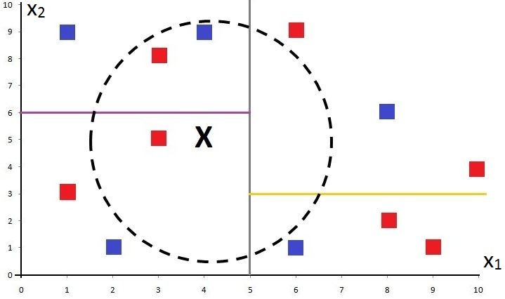
If we repeat the process, the algorithm takes a different attribute. In our example, the only variable left is X₂, so the algorithm considers X₂ and takes its median to divide a branch of the tree into two halves with an equal number of points on each side. Here, the value 6 is taken on the y-axis to divide the branch with X₁<5 into two equal halves.

The same plot, now also showing a horizontal purple line at X2 equals 6 dividing the left-hand region (X1 less than 5) into two halves

We do the same for the other branch of the tree, and this time a value of 3 is taken as the median to divide that branch’s data into two equal halves.

The same plot, now also showing a second horizontal yellow line at X2 equals 3 dividing the right-hand region (X1 greater than or equal to 5) into two halves

By doing this, we’re able to limit the number of data points in each “section” or branch of the tree. We continue until a predetermined amount of data, M, is obtained in each section/branch. As the dataset is divided in half at every step, the maximum depth of this tree cannot be greater than log₂ N.

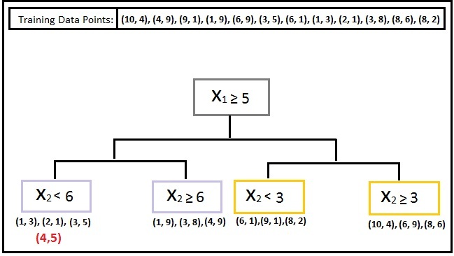
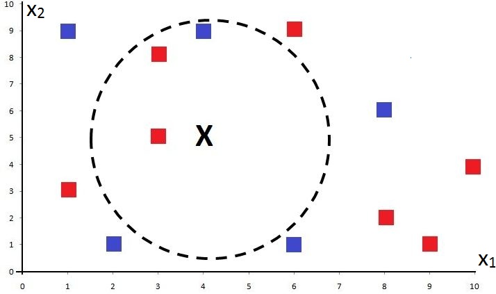
The full tree diagram with the root node X1 greater than or equal to 5 splitting into four leaf nodes based on X2 less than 6, X2 greater than or equal to 6, X2 less than 3, and X2 greater than or equal to 3, each listing its three or four contained training points

We can now look at our X point and see that the number of training points it needs to be compared with is 3, much less than the total of 12 training points.

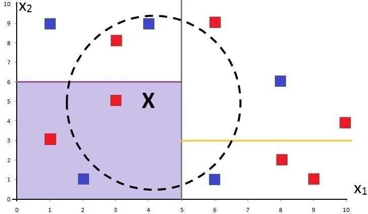
The plot with the lower-left quadrant (X1 less than 5, X2 less than 6) shaded purple, showing the 3 training points sharing a leaf with the testing point X

This also points to a potential problem. We can see that this method misses some actual nearest neighbours - the two points above X (a Red and a Blue square) that lie just outside the shaded region. As the algorithm divides the data points into sections, a training data point - no matter how close it is to the testing point - will not be considered a potential neighbour if it falls into a different section.

This method missing some actual nearest neighbours is one of its biggest disadvantages, but it’s the cost we pay to save time during the testing phase.

Locality-Sensitive Hashing

This method is used when the data has a lot of features but is not sparse, and is in some ways similar to K-D Trees. Let’s understand the process of LSH using the same dataset used to explain K-D Trees. LSH, just like K-D Trees, cuts the dataset into regions; however, this time medians are not used to divide the dataset. Instead, we draw random lines to divide the dataset (we’d use hyperplanes instead of lines when the data has more than 2 dimensions/features).

Let’s say the algorithm draws a random grey line dividing the dataset into two regions.

The same scatter plot with a single random diagonal grey line drawn across it, splitting the dataset into two regions

The algorithm continues and introduces another random line to divide the dataset such that we end up with 4 regions.

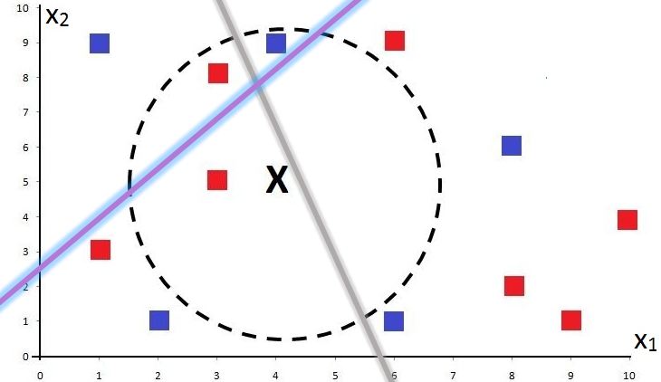
The same plot with a second random diagonal line (blue/purple) added, crossing the first line and creating four regions

If we continue and draw another line, we end up with even more regions. Therefore, if we draw K lines, we get 2^K regions.

The same plot with a third random diagonal line (yellow) added alongside the previous two, creating additional regions across the dataset

Each training and testing data point falls into one of these regions, and this division of the data space into regions helps reduce the time needed to complete the testing operation. However, just like K-D Trees, this method will also miss some actual nearest neighbours.

Inverted Lists

This works as the opposite of K-D Trees and is used when the data has a lot of features and is sparse. So if we have a lot of features - which is generally the case when working with text data - this method is used to reduce the number of training samples we compare against.

Let’s say we have data with 5 sentences:

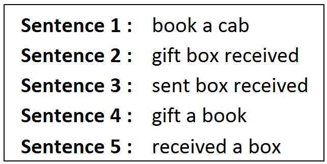
Five labelled sentences: Sentence 1, book a cab; Sentence 2, gift box received; Sentence 3, sent box received; Sentence 4, gift a book; Sentence 5, received a box

When we label these sentences as either spam or an actual personal message and convert them into a dataset, each word becomes a feature, and the data looks something like this:

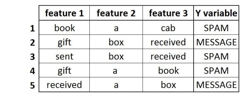
A table with columns feature 1, feature 2, feature 3 and Y variable, listing the words of each of the five sentences and their SPAM or MESSAGE label

As each word will not be repeated across every sentence, this causes sparseness. Notice how feature 2 is less sparse than feature 3, where only once does the word “received” get repeated. Therefore, a concept known as the Inverted List is commonly used with text classification problems, where for a word, all the instances of that word in the dataset are noted. So if we have the word “book”, rather than using all the features, we can say that this word occurs in sentence 1 and sentence 4. For all the words, the dataset then looks like this:

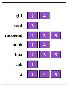
An inverted list showing each distinct word (gift, sent, received, book, box, cab, a) mapped to the sentence numbers in which it occurs

In these methods, only the instances where the word occurred in the dataset are remembered. In a binary sense, each word with a non-zero value is remembered, while all the other 0 “non-existing” instances are removed. So if we have a new test sentence - ‘cab gift’ - the KNN algorithm doesn’t have to look at all the sentences. Rather, it will only compare the test sentence with those instances where the words of that test sentence occur.

So our KNN algorithm will merge these two instances and consider Sentences 1, 2 and 4, classifying the test instance (which, for K=3, will be SPAM). Since the words of this test sentence don’t exist in the other training sentences, this procedure saves time, as the other sentences won’t be used for comparison. Unlike K-D Trees and Locality-Sensitive Hashing, this method doesn’t miss actual nearest neighbours and saves a lot of time - however, it only works for sparse datasets.

All these methods help reduce the time taken by the KNN algorithm during the testing phase. Each can be used depending on the situation: K-D Trees and Inverted Lists work well for sparse datasets, while Locality-Sensitive Hashing can be used with datasets that are not sparse. All of these methods aim to reduce processing time, and applying them makes KNN more efficient.