// time series

Smoothing Techniques and Time Series Decomposition

Time series models are created when we have to predict values over a period of time, i.e. forecasting values. There are multiple techniques to do this. In this blog, some medium-level techniques are discussed, such as Exponential Smoothing techniques and Time Series Decomposition.

Exponential Smoothing

Exponential smoothing is also known as the ETS Model (Error, Trend, Seasonal Model) or the Holt-Winters Method.

Smoothing methods have a prerequisite, which is that the data is 'stationary'. Therefore, to use this technique, the data needs to be stationary, and if it is not, the data is converted into stationary data. If such conversion doesn't work or isn't possible, then other techniques such as Volatility models are used, where techniques such as ARCH, GARCH and VAR are applied (the same applies when using ARIMA methods).

There are various kinds of exponential smoothing, such as Single Exponential, Double Exponential and Triple Exponential Smoothing.

The formula for exponential smoothing is Y_t = f(Y_t−1, E_t−1), where Y_t is the current value, Y_t−1 is the last time period's value, while E_t−1 is the last period's error.

In simple words, the current time period's value is a function of the past time period's value and the past time period's error. Also, note that if there is a pattern in the error, it means that the model is not correct, as the errors should be independent.

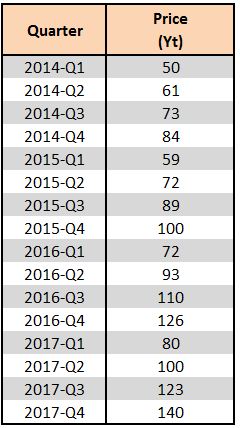
We will use a dataset to understand how exponential smoothing works. Below we have a dataset where the actual values (Price) are represented as Y_t.

Single Exponential

In exponential smoothing, the forecast values are represented as F_t, while the difference between Y_t and F_t is represented as E_t (error). Here the current time period is a function of the past time period as well as the past error (Y_t=f(Y_t−1, E_t−1)).

The formula for exponential smoothing is:

F_t+1 = F_t + α(Y_t − F_t)

where F_t+1 = forecast for the current period, F_t = last period's forecast, and α = Smoothing Constant (a value between 0 and 1).

Another way of writing the same formula is:

F_t+1 = αY_t + (1 − α)F_t

where F_t+1 = new forecast, αY_t = alpha multiplied by the last actual value, and F_t = last forecast value.

To implement either of these formulas we use the above-mentioned dataset. We must note that as of now we are not sure of the correct value for alpha. Smaller values of alpha lead to more detectable and visible smoothing, while a larger value leads to faster responses to recent changes in the time series but provides a smaller amount of smoothing. We can determine the value of alpha through trial and error, selecting the value that provides the minimum error, or use various optimization techniques available in statistical software which automatically identify the correct alpha. For now, we take the alpha value at 0.2 and do the following calculations.

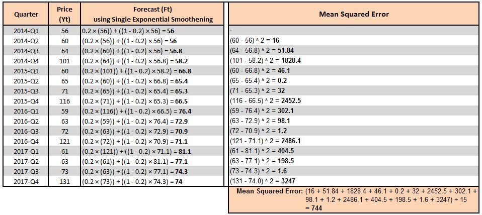
Here we use the formula F_t+1 = αY_t + (1 − α)F_t.

Notice that for the first entry, 2014-Q1, we don't have any previous forecast value, so we take the previous forecast value to be the actual value, i.e. F₁=Y₁. Therefore the first actual and forecast values are the same. The second forecast value is also nothing but the previous actual value. Thus, generally, the forecast is started from the second entry, where the second forecast value is assumed to be the previous actual value. We then use the formula and take the previous actual value and forecast value to predict the current forecast value. We then calculate the mean squared error of these values and arrive at an MSE of 744.

Double and Triple Exponential

In Double Exponential, two past time periods and two past errors are considered, and here we need α (alpha) as well as β (beta). Similarly, in Triple Exponential, we consider the past three time periods, requiring alpha (α), beta (β) as well as gamma (γ).

Thus, if we forecast through the above-mentioned single exponential smoothing method and then perform another single exponential smoothing on top of it, the result will be something like double exponential smoothing. Similarly, if we continue and take another single exponential smoothing, we will end up performing triple exponential smoothing. Here, alpha, beta and gamma will be unknown, and this is where ETS models come in, using the Holt-Winters method to determine them. One must note that single exponential smoothing requires stationary data, double exponential is able to capture linear trends, while triple exponential can handle a wider variety of data.

Smoothing techniques are very helpful; however, there is another medium-level technique which is commonly used, known as Time Series Decomposition.

Time Series Decomposition

Time Series Decomposition is a pattern-based technique. As mentioned in Introduction to Time Series Data, the four main components of time series data are Trend, Seasonality, Cyclicity and Irregularity.

Thus, to put this in a formula, we can say that the current time period is a function of these four components, i.e. Y_t = f(T_t, S_t, C_t, I_t), where Y_t is the current time period, T_t is trend, S_t is seasonality, C_t is cyclicity and I_t is irregularity.

There are two types of Decomposition Models:

1) Additive Model: Y_t = T_t + S_t + C_t + I_t. Here Y_t is the sum of the four independent components: Trend, Seasonality, Cyclicity and Irregularity.

2) Multiplicative Model: Y_t = T_t × S_t × C_t × I_t. Here Y_t is the product of the four independent components: Trend, Seasonality, Cyclicity and Irregularity.

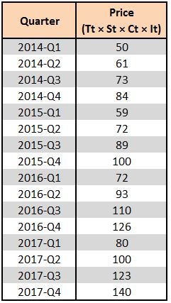
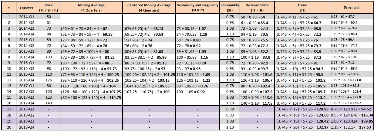
To understand Time Series Decomposition, we will use a dataset and perform time series decomposition on it. For example, we have the following dataset, where Y_t is the price variable. Thus, if we are considering the Multiplicative Model, then we can say that the 'Price' variable = T_t × S_t × C_t × I_t. We now start with creating a multiplicative time decomposition model.

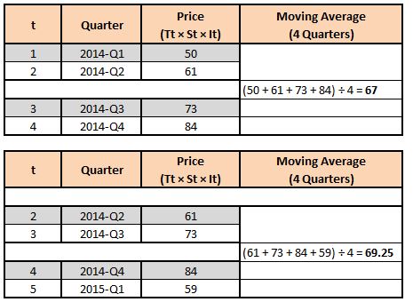
Step 1: We first start by adding a variable 't', which will be nothing but a time code that will be useful in the upcoming steps.

Step 2: We have four independent components in our data: Trend, Seasonality, Cyclicity and Irregularity. We can confirm this by visualizing the data and creating a line graph.

We can see that there is an upward trend along with cyclicity, where the price peaks at every fourth quarter of the year. There is also some irregularity present. However, cyclicity is something that is rarely found, and as the data available to us is limited and estimating cyclicity needs data from the past 6-7 years, we do not include the cyclicity component when performing short-term forecasting. Thus, our Y_t is made up of three components: Trend, Seasonality and Irregularity.

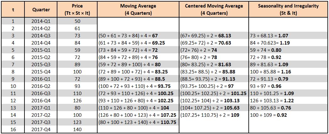
Step 3: In this step, we 'smoothen out' the data. As shown above, the data has seasonality and irregularity, and we can smoothen it out by removing the peaks and slumps. This is done by taking the moving average. As our season is made up of four quarters, we consider four periods to calculate the moving average. Below we have calculated the moving average, starting with the third row and considering the four quarters to come up with the moving average values.

Notice that we don't compute the moving average for the last row (2017-Q4), as we don't have a 17th value required for computing the moving average.

Step 4: We are required to compute a Centered Moving Average, as in the above step we took the moving average of an even number of periods. To understand this intuitively, consider the first moving average that we computed, which is 67 (2014-Q3); this technically should represent the centre of 2014-Q1 to Q4, as we averaged the values of these four quarters. Therefore, the value 67 should lie between 2014-Q1, 2014-Q2 and 2014-Q3, 2014-Q4, and this should continue throughout, where the values should represent the exact centre of the four periods.

Thus, as of now, the value 67 doesn't represent 2014-Q3 but rather represents the value between 2014-Q2 and Q3. We don't have a centred average, as the values fall between the numbers being averaged, which is always the case when the time period taken for computing the average is an even value. If the time periods were an odd value, we wouldn't have required the additional step of centring the averages; however, here we do. Thus, we compute the Centered Moving Average, where we average the two adjacent values of the moving average to return to the centre.

For example, if we find the mean of the 2014-Q3 and 2014-Q4 values, we can use this value to represent 2014-Q3. Notice that we don't calculate the centred moving average for 2017-Q3, as we don't have the moving average for 2017-Q4.

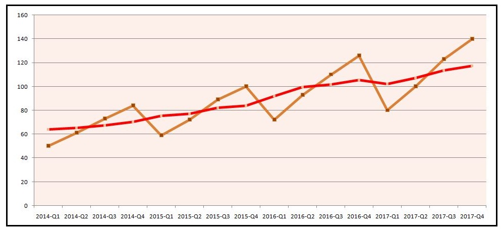
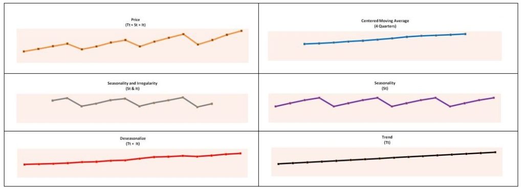
Now, these centred moving averages can be plotted, and this provides us with a 'baseline' which represents the data devoid of seasonality and irregularity.

Step 5: We can look at the above graph and understand that the difference between the orange line (having all three components) and the blue baseline (data devoid of seasonality and irregularity) can be used to extract seasonality and irregularity.

We know that as per the multiplicative model, Y_t = T_t × S_t × C_t × I_t. As we don't have any cyclicity, Y_t = T_t × S_t × I_t.

Now, to extract the seasonality and irregularity component, we simply divide Y_t by the Centered Moving Average. The idea is that dividing the original data points by the 'smoothened' data points provides us with the seasonality and irregularity component.

To put this in context, the value 1.07 (the value of S_t & I_t for 2014-Q3) means that in 2014-Q3, the seasonality and irregularity component was 7% above the smoothed data, or baseline, while the value 0.80 (the value of S_t & I_t for 2015-Q1) means that for this time of year, the seasonality and irregularity components were 20% lower than the baseline.

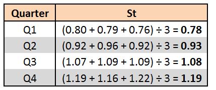
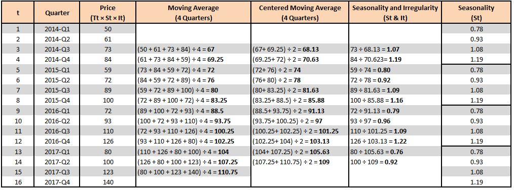
Step 6: In this step, we extract the Seasonality component from the Seasonality and Irregularity column. For this, we come up with a Seasonal Index. We know that each of our 'cycles' (not to be confused with cyclicity) is made up of four quarters. Thus, to find the Seasonal Index values, we average the Seasonality and Irregularity values for each quarter, and this way we get rid of the irregularity component.

We add these values to the main table. With the Seasonal Index value, what we mean is that, for example, in 2015-Q1 the Seasonality Index is 0.78, which means the seasonal component is 22% lower than the baseline, while it is 19% more in 2015-Q4.

Step 7: This step is known as Deseasonalizing. Until now, we first computed the baseline, which was devoid of seasonality and irregularity. Using it and the original values, we extracted the seasonality and irregularity. Then we isolated seasonality, and now, as we have seasonality and know that Y_t = T_t × S_t × I_t, we use the following formula: T_t × I_t = Y_t ÷ S_t.

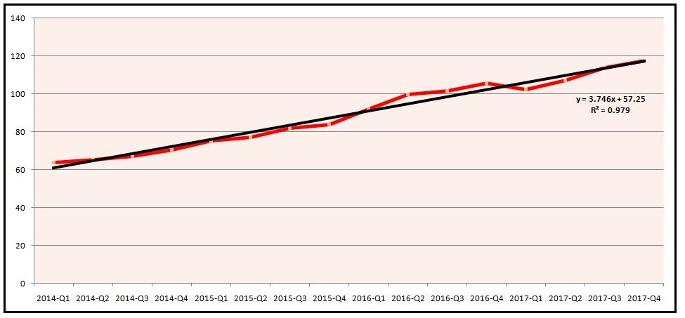
If we plot a line graph of the Price variable and the deseasonalized variable, we can see the difference. The orange line (Y_t) has all four components, while the red line (the deseasonalized line) is devoid of peaks and slumps, as the seasonal component has been removed from it. As this line trends upward, it means there is a trend component in it; however, the irregularity component is also present.

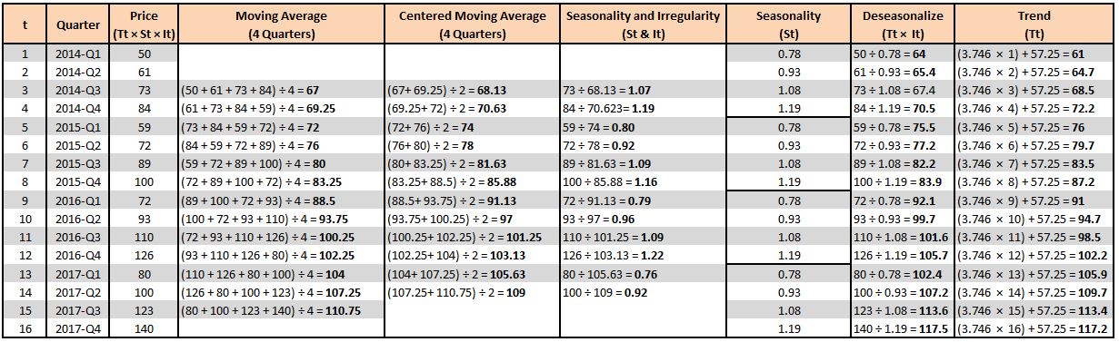
Step 8: So far we have isolated the seasonality component. In this step, we extract the trend component, which we do by running a simple linear regression where the deseasonalized variable is our Y variable, while the t variable is our X variable. The regression provides us with the following equation: 3.746x + 57.25. Here 3.746 is the coefficient of the x variable, while 57.25 is the intercept. We use this equation to come up with the values for our trend line, where for the first data point, x will be 1, for the second it will be 2, and so forth.

Thus, the trend line is nothing but a simple regression where the x variable is the time code, while the y variable is the deseasonalized values. When we compare the deseasonalized line with the trend line, we can see some differences, which are due to the irregularities present in the deseasonalized line.

Step 9: Until now, in the time series decomposition method, we have successfully extracted the seasonality and trend components and got rid of the irregularities. Comparing all of them: the orange line represents Y_t, which has all three components (cyclicity is not being considered in this example); the blue line represents the baseline, which we compute using the centred moving average and which provides a baseline devoid of seasonality and irregularity to some extent (this cannot be considered a trend line); we then use this baseline to derive the grey line, which has the seasonality and irregularity component, and use it to extract the seasonality line (purple line); the seasonality component is then used to isolate the irregularity and trend (red line, deseasonalized), and by running a simple regression on the deseasonalized values we arrive at the black line (trend line).

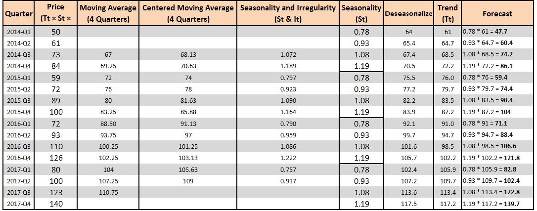
We now make predictions through the multiplicative model, where Y_t = T_t × S_t. We first forecast the values for the time periods for which we already have actual data, as this helps us use an error measure.

If we want an error measure such as the Mean Squared Error, we can subtract the original values from the forecasted values, square them, and take an average of these values, which in our case comes out to an MSE of 6.2.

Now we also forecast for the upcoming four quarters. We do this by using the seasonality and trend components and multiplying them, which gives us the forecasted values. If we forecast for the next two years (2018 and 2019) and plot the actual and forecasted values, we can understand the forecasted values more visually.

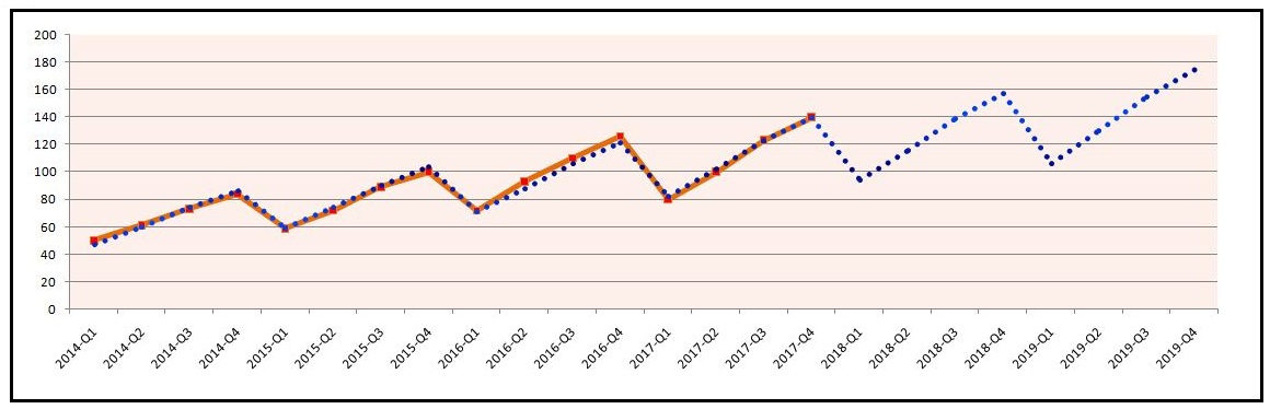
We can see that our multiplicative time decomposition model is able to forecast values with a lot of accuracy. We can also use other methods, such as the Additive Model; if the data has a minimal trend but has seasonality, the additive model is suggested, whereas if the data has sizable seasonality and trend, the multiplicative model is generally better.

Time Series Decomposition and ETS models are medium-level techniques for forecasting values and should be used if the data has seasonality and trend. There are other high-level methods, explored in the next blog, where techniques belonging to the ARIMA family are discussed.