// dimensionality reduction

Factor Analysis

Factor Analysis is a classification technique which works in an unsupervised environment. It is used to identify the similarity between the various features and form groups of them, which it does by extracting the maximum common variance from all variables. The most common usage of Factor Analysis is for data reduction, through which it helps in reducing the features by identifying variables that are highly correlated to each other. To perform factor analysis, we require continuous variables (numerical, interval scaled) with a good sample size.

Factor Analysis can be complex to understand without an example, so an example will be used to explain the whole process of factor analysis.

Introduction to an Example

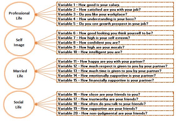
We have a dataset where our dependent variable (Y_variable) is ‘happiness’, which is a binary categorical variable having two values, 0 and 1, with 0 denoting ‘unhappy’ and 1 meaning ‘happy’. We have 20 independent variables, and it is required to reduce this number of features. Suppose we get to know how these 20 independent variables were created - turns out that these 20 variables came from 4 separate surveys, where each survey had 5 questions providing a score of 0 to 5 for a response.

(For example, 5 of the independent variables belong to a single survey: Survey-A, that had 5 questions.)

Latent Variable

Each of the above questions is not random but is a part of a larger construct, and this construct is known as ‘Value’, while each of these questions is an ‘observed variable’, as their values are measured, i.e. they are actually observed from the responses. All these observed variables here represent a ‘value’, and this value is called an ‘unobserved variable’ or Latent Variable, and they are called so because these variables are not measured directly but rather are pointed out / indicated by the observed variables. Thus in this example we can easily calculate that there are four latent variables, with each latent variable having 5 observed variables; however, in real life the required information to calculate this is not known, and a statistical analysis is required to find how many values go well together in one construct, and if there is a need for having more than one construct, then how many values in one construct are different from values of the other, making their respective construct unique. This statistical analysis is known as Factor Analysis.

Coming back to our example, suppose we have no information about the underlying construct and all the 20 variables seem independent to us. We now, from these multiple observed variables, have to find similar patterns of response associated with a latent variable. In our example, we will find these constructs statistically by using factor analysis in a number of below-mentioned steps.

EFA and CFA

There are broadly two kinds of factor analysis, Exploratory Factor Analysis (EFA) and Confirmatory Factor Analysis (CFA). EFA is what has been discussed so far, where the variables that are highly correlated to each other are grouped. This group is known as a ‘factor’. Once this factor is created, it looks for another set of variables and groups them, making another factor. The number of factors that are to be created depends on the analyst, and N (number of observed variables) number of factors can be created (i.e. one factor for each observed variable). This N number is decided based on a number of factors (discussed later in this blog).

CFA is used when we already have an idea about what the latent variables are and which of the observed variables belong to which latent variable. For example, we have ten variables where five of them seem to be related to education, such as - How important are formal studies to you? Are you satisfied with the current method of examination? etc. - while the other set of variables clearly seems to be dealing with sports, such as how important sports are, how satisfied are you with the current situation of sports training? etc. Here we can easily guess that there seem to be two latent variables; however, to prove this statistically, we require performing hypothesis testing, and this is where CFA helps.

In this blog post, we’ll be concerned with EFA only, as we presume that we have no idea of what these latent variables are and how many there are in the dataset.

Extraction and Factor Rotation

The whole idea of factor analysis is that by having all the variables, we have 100% data, which in statistical terms means 100% variance. When we reduce the number of variables and still try to cover 70-80% of data, we are in a way trying to capture 70-80% of the variance; therefore, the target is reducing the maximum number of variables and at the same time retaining most of the variance provided by the variables. For this, we group the variables into groups known as factors. However, we initially don’t have any idea about how many of these groups are to be created, and in most statistical software, a hit-and-trial method is used where, as a thumb rule, we assume that each factor has 4 or 5 variables, thus we divide the total number of variables by 4 or 5, and the output is what becomes the initial number of factors required for performing factor analysis. In our case we take 20 ÷ 5 = 4, therefore we decide to perform a factor analysis with a four-factor solution.

Now, to group all the variables into 4 factors, Factor Analysis uses a method known as Extraction. In this process, it first finds the largest group of variables that are highly correlated to each other and creates a group from them, and this group (factor) explains most of the variance of all the variables in the analysis. Then it proceeds to find the next batch of highly correlated variables, with this second factor explaining the second most variance in all the variables, and so on. In our example, we take a four-factor solution, so we end up with four of these factors.

The output looks something like this:

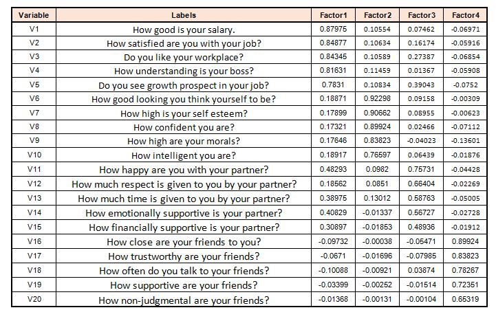
Here each of these analyses or rows is a factor loading. The values of these factor loadings are very similar to correlation coefficients, where a higher value means that variable highly defines that group (factor). This output is generated through extraction; however, there are many ways through which extraction can be done, such as:

• Principal Component Analysis
• Maximum Likelihood
• Image Factoring

One of the most commonly used methods of extraction, which will be discussed briefly here, is Principal Component Analysis. In Principal Component Analysis, the maximum variance is extracted and is placed in the first factor. Then, for constructing the second factor, the variance explained by the first factor is removed. This process is done for all the factors. This method of extraction is so common that it is the default method of extraction for factor analysis in most statistical software.

As mentioned above, the factors need to be distinct from each other, and in order to do this the original variable space is rotated - this is known as Factor Rotation. There are many ways to rotate the spaces. The most common method of rotation, commonly associated with Principal Component Analysis, is VARIMAX, where we extract the maximum variance by rotating the principal axis. This method of rotation is also called orthogonal rotation. Other methods of rotation are also there, such as PROMAX, also known as oblique rotation, where the assumption that the factors are orthogonal to one another is dropped, creating factors that are correlated with each other.

Both these methods of rotation are important and can be used; however, PROMAX is generally considered to be better, as in the real world factors will be moderately correlated to each other and won’t be as starkly unique as presented by VARIMAX; however, VARIMAX is easy to score and interpret, and thus has its own set of advantages. Other rotational strategies are QUARTIMAX, EQUAMAX, etc. In general, PCA is followed by VARIMAX, with the former constructing latent factors while the latter makes the factors distinct.

In the end, one must remember that the aim of all such rotational strategies is to obtain a clear pattern of loading, so that it becomes easy to mark and distinguish the high loadings from the low loadings in each factor (see below image).

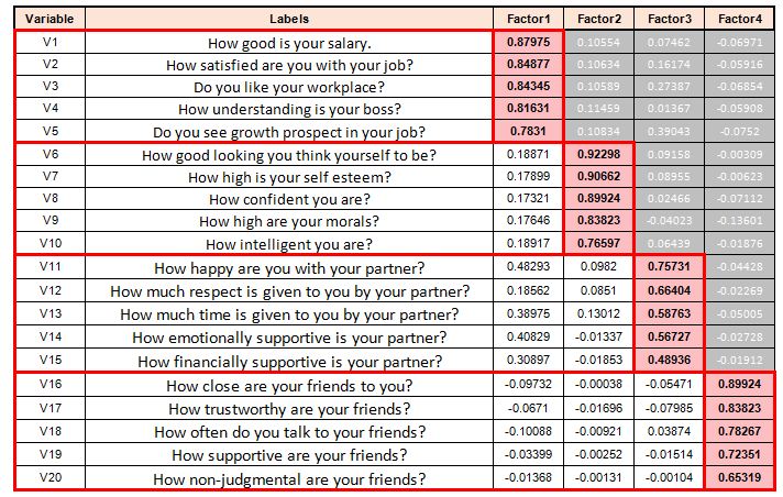
However, if such factor rotation methods are not used, then we would have numerous factors that will all be based on some variation found in the highly correlated variables, and because of this, it will never be able to reach the actually varied, less correlated variables.

PCA v/s PCA

In the blog Principal Component Analysis, its use was explored as a dimensionality reduction technique; however, here in Factor Analysis, which as such is not a feature reduction method, we are using principal components. It can be confusing to distinguish between these two uses of PCA, especially when most statistical software uses Principal Component Analysis as the default method of extraction for Factor Analysis. To clarify, you must understand that the Principal Component Analysis discussed in the earlier blog is an independent analytical method, a feature reduction technique generally used when variables are highly correlated, which are reduced to a smaller number of principal components that account for most of the variance of these variables. Principal Component Analysis here can be seen as simply a mathematical transformation.

On the other hand, in this blog, Principal Component Analysis is used merely as a factor extraction method, i.e. a tool to construct latent factors. Here we estimate factors, and arbitrarily select the variables for future modeling purposes. Here, Factor Analysis is more of a statistical technique to classify the variables and select variables that seem relevant by maximizing their variance. Thus they are two different models that can be used for feature reduction, wherein PCA the components are orthogonal linear combinations where the total variance is maximized, while in FA (Factor Analysis), PCA can be used to extract factors, but here the factors are linear combinations where the shared portion of the variance is maximized.

Determining Number of Factors

As mentioned in the beginning, Factor Analysis requires some hit and trial before we can get an optimal solution. Till now, we decided to perform EFA, presuming that we don’t have any information about the underlying constructs. We then started our exploratory factor analysis by selecting a number of factors based on a thumb rule of the number of variables divided by 5 (considering each factor will have 5 variables). We then chose the method of extraction to create the latent variables and decided to go with PCA, and for example decided to choose orthogonal factor rotation as a means to make the factors unique from each other. All this information, when input into a statistical software, produces a Table of Communalities, which can be used for deciding the number of factors that has to be used.

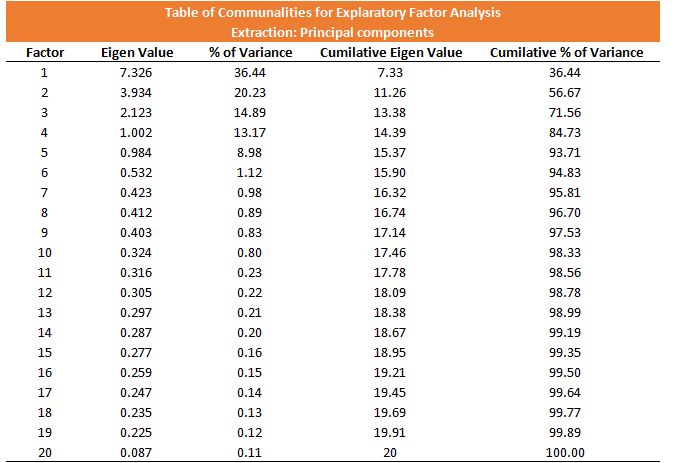
The understanding of the Table of Communalities is very important to effectively decide the number of factors. Here the first column is for the number of factors. As mentioned earlier, we can have as many factors as there are variables in observation. In the second column, Eigenvalues are provided. The third column is derived from eigenvalues only, which indicates the % of the variance. We can see that Factor 1 has the maximum variance - this means that we have successfully extracted maximum variance (36%) in the data on this factor. The second factor accounts for 20% of the variance, and this number gradually decreases for each of the other factors. The second-last column explains the cumulative eigenvalue, while the last column has the cumulative percentage of variance explained by each factor.

We first understand these columns intuitively. The factor column means how many factors explain the variance. If we go with 1 factor, i.e. the minimum amount of factor, then it will provide us with a factor where all the variables are grouped together. If we choose variables from this factor, then we can decrease the multicollinearity, but we will be forcibly combining variables that are essentially different. Also, we will end up losing a lot of information, as the total variance explained by this factor is only 36%. If we increase the number of factors by 1, then we also increase the chances of multicollinearity but also increase the variance that can be explained. Also, we ‘free’ the variables that were forcibly grouped together. However, if we keep on increasing the factors, then the variables that should ideally be in a group will start to break away, and selecting variables on a common ground will become difficult, and this will eventually cause multicollinearity, destroying the very reason for which factor analysis was performed, i.e. feature reduction. Notice how the last factor has 100% cumulative variance, i.e. if we take all 20 factors, we won’t lose any information. Thus we can use eigenvalue as a synonym for multicollinearity and variance as a synonym for data captured. Now we have to consider the trade-off, so that we can strike a balance between multicollinearity and data captured.

The Kaiser criterion

According to this criterion, we retain only that number of factors where the eigenvalue is greater than 1. The idea behind this is that if a factor explains less than the variance carried by a single variable - in our 20-variable example, less than 5% (1÷20) of the total variance - then probably it may not be as useful. However, in common practice, the ideal eigenvalue is considered to be the one which is just below 1. This is done to keep the aspect of multicollinearity in control.

Scree Plot

We can also decide the number of factors by plotting the eigenvalues on a simple line plot. The method involves finding where the smooth decrease of eigenvalues levels off, and factors around that ‘elbow’ can be considered.

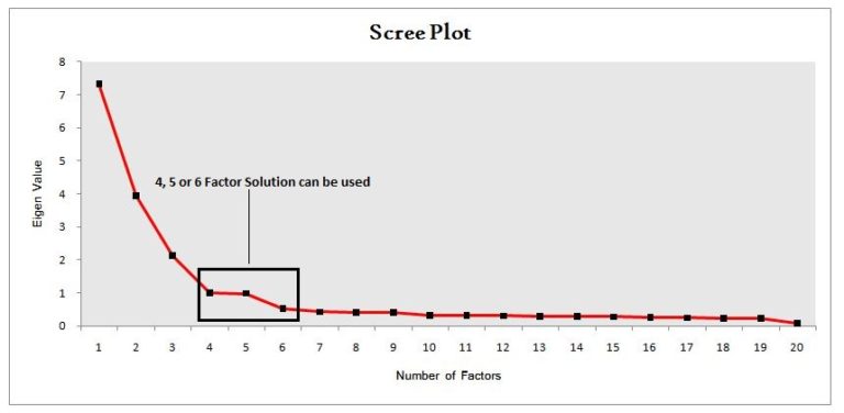
In our example a 5-factor solution can be used; however, in real life, hit and trial with different factors is required.

Selecting Variables

The final step includes picking variables from each factor. Here we group the variables that have the highest factor loading for that factor and choose the relevant variables from them. This part is very subjective, and the variables that are selected from each factor depend on various factors, such as business scenario, client demand, etc.

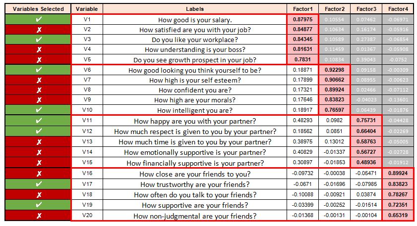
In our example, we can see that job-related aspects play a major role and emerge as the strongest factor, explaining around 36% of the variance, with items such as the salary earned and the satisfaction with the job having strong loading. Growth prospect has relatively weak loading; however, the variables that we select are subjective and are based on numerous factors.

Thus we are able to group all our variables into ‘factors’ that have some common notion/background to them.

Factor Analysis is a classification technique, but we can use this technique to pick variables by forming groups of correlated variables that have some meaning to them. This method requires a bit of to-and-fro but is useful when we require reducing the number of variables and need to make some arbitrary decisions.