// dimensionality reduction

Principal Component Analysis

Principal Component Analysis is a modeling technique which works in an unsupervised technique. Unlike the other methods discussed in this section such as Factor Analysis, PCA is an unsupervised dimensionality-reduction method that focuses on extracting the maximum variance from the features. There are various variants of this unsupervised learning algorithm such as Kernel PCA and Independent Component Analysis; a related supervised counterpart is Linear Discriminant Analysis (LDA).

Overview

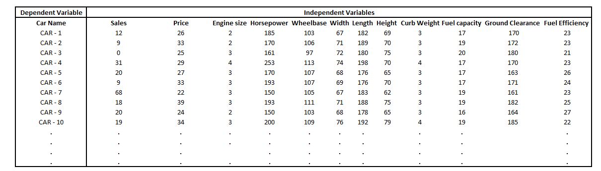
Before getting into the details and nitty-gritties of the whole working process of the PCA, let’s first have a brief idea of its working. Imagine we have a dataset where we have various features of a car as the independent features and as the dependent variable we have the price of the car (a numerical variable) or we can have the name of the car (a categorical variable). However, these independent features have some underlying groups which are very similar to each other. For example, certain features are related to the dimensions of the car, such as the size of the tires, the ground clearance, the height of the roof of the car, the overall width of the car, overall height of the car, and these features can be correlated to each other - for example, the size of the tire can be highly correlated to the ground clearance, thus not adding much information. Similarly, other groups of features can be there. Suppose if the dataset has hundreds of such features, it will become very difficult to determine these types of underlying groups, as we can’t observe the differences from the outside. To find the groups, for example, we create a scatter plot using two features, height and weight of the car, and find that these two variables are positively correlated, with certain cars having very high correlation (higher height and consequently higher weight) while some of these cars will have lower relation (high height but not much weight); however, when seen on an overall basis, these two variables show a positive correlation. Positive correlation here basically means that they are indicating similar things, and a negative correlation (for example, in the case of engine size and mileage, where with an increase in the size of the engine, the mileage will decrease) means that these two features are similar but in an opposite way.

Now, if we have to analyse one variable, it can be done using a simple line where data points will lie on a line, and we can easily see the data points that are distinct from the others and how these data points affect the dependent variable. If we have to find the relationship between two data points, it is a 2-Dimensional problem (2-D), and we can use a scatter plot where the height or Y (vertical) axis can represent one variable while the breadth or the X (horizontal) axis can represent the second variable, and by looking at it we can find if these variables are related to each other or not. Similarly, if we were to find the relationship between three variables, we can then use a more fancy 3-D plot, with depth being the third axis used for representing the third variable; however, this will cause a problem for us, as analysing such a graph will become very difficult, as we will require rotating such a graph to find the relations in the features.

If we were to analyse 4 or more variables simultaneously, we will have to make a graph which will have an axis for each feature that cannot be contemplated by a human mind.

So, for now, we have two options if we have to find relationships between, for example, 100 variables: either make thousands of 2-D plots or make a very ridiculous plot which cannot be comprehended by a human mind. The answer to this question is PCA. We can create a PCA plot which converts the correlations or the lack of correlations among the features into a 2-D graph, clustering the features that are highly correlated to one another. In our example, we may find groups of features which we can then categorize into ‘Dimensions of Car’, ‘Performance of Car’, ‘Power of Car’, etc.

In other methods, the feature which doesn’t provide much information is dropped, i.e. if we have two variables that are highly correlated, we can drop one of these variables. However, if the features are not statistically independent, a single feature could therefore be representing a combination of multiple types of information by a single value. To understand this better, let’s take an example of image classification, where we use red, green and blue components of each pixel of an image to classify the image. The process includes capturing of the data by different image sensors, where image sensors that are most sensitive to red light capture that colour but also capture some blue and green light. Similarly, sensors that are most sensitive to blue and green light also exhibit a certain degree of sensitivity to red light. Thus the R, G, B components are as such co-related, but it is not tough to understand that even though they are co-related, each component is important and provides information, and no feature can be dropped, as if we remove the Red component, we also end up removing the information about the G and B channels. Thus, to eliminate features, we cannot just eliminate redundant features but have to transform the feature space such that the underlying uncorrelated components are obtained.

PCA uses this correlation to transform the data into a new space with new uncorrelated dimensions by linearly combining the original dimensions, thus creating a new set of features which is a linear combination of the input features. This is done by rotating the coordinate system in such a way that the new dimensions are completely uncorrelated and represent only the different and independent aspects of the input data. Principal Component Analysis thus reduces higher vector spaces into lower orders through projections, compressing the dimensions and making visualization easy, so if we have data in 3 Dimensions (for example, R, G and B components), PCA converts it into 2 Dimensions by finding the plane which captures most of the information. This data is then projected on a new axis, and this causes a reduction in dimensions. When the projection of components happens, the new axis is created to describe the relationship, and they are called the principal axis, and the new features are called principal components. These new dimensions are provided with a score by PCA, with high dimensions having a large amount of information but providing less reduction of the dimensionality, and the lower dimensions having a lesser amount of data, as data is in a closed region, making it tough to discriminate data samples from each other but reducing the dimensionality to a great extent.

PCA in Detail

We have to first consider a dataset. For example, we have a dataset where we have the car’s name as the dependent variable while the independent variable contains the various information about the car, and we want to reduce the dimension of the data.

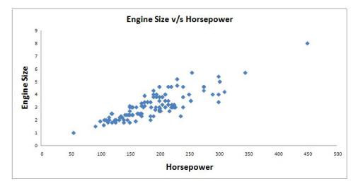
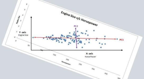
We can create a 1-dimensional plot, which is nothing but a number line where we can consider only one variable. However, this is of not much use to us in reducing features. We can create a 2-D graph where we will have 2 axes and we can plot data from 2 variables. Here we use Engine Size and Horsepower and find that they have a positive co-linear relationship.

If we have to create a plot to represent three variables, for example Length, Engine Size and Horsepower, we then will have to create a 3-D graph, which then will be required to be constantly rotated to find the relationships (which will be difficult). Here the X axis represents Length, Y represents Engine Size, while Horsepower is represented on the Z axis (Depth).

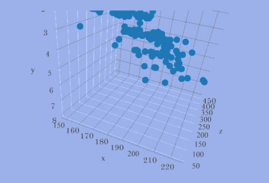
If we have to find relationships among these three variables, we will have to draw lines perpendicular to each axis for each data point to find where they all meet, and have to do this for all the observations to be able to finally come to any conclusion. Thus this fancy graph is of not much use to us. To find relationships among 4 or more variables, the plot won’t be of any more help.

For example, we have hundreds of features, and we have to find those features which are the most important, but for understanding how PCA can help in reducing hundreds of features, we take a much simpler example where we have 2 features and we require reducing them without dropping any variable, i.e. minimizing the loss of information. If our 2-D graph (having 2 variables) has variation in only one feature while the other feature has very little variation, then the variation in the data can be said to be from left and right.

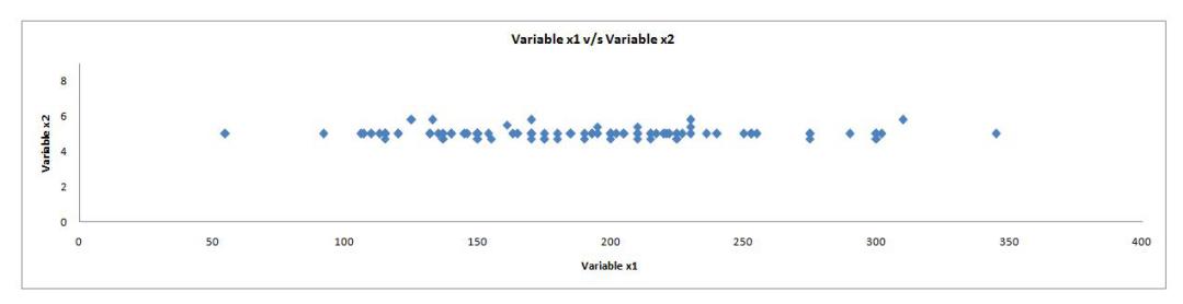
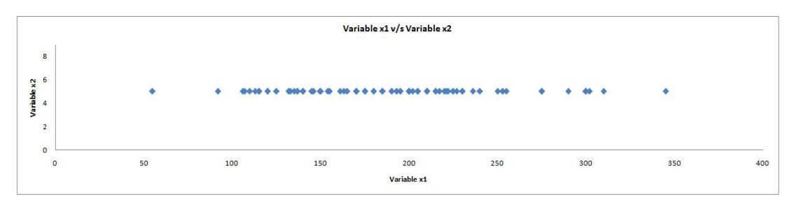
Here only the variable x1 has variance, while the variable x2 has less variance. If we remove the little variance found in the x2 variable, we will have a plot that would look something like shown below, which as such can be represented as a 1-Dimensional graph (a number line). Here we converted 2-Dimensional data into 1-Dimensional data without losing much information (hereby information we mean the variance that we flattened out), as in both the graphs it is clearly visible that the important variation is from left to right, i.e. the axis where variable x1 is plotted, thus answering our question of which variable is more important - and here the variable x1 is of more importance.

Thus each feature adds another dimension; however, each of these dimensions has different variance, therefore some of these dimensions are more important than the others. PCA works on similar lines, as it takes in data from a lot of dimensions and flattens it to lower dimensions (2 Dimensions for visualization) by finding meaningful ways to flatten the data by focusing on things that are different between the features.

Coming back to our previous example of Engine Size and Horsepower, we can see that our data points are spread out along the diagonal line, as the maximum variance in this data can be found by finding the two extreme data points of this feature (Horsepower). However, the dots are also spread out above this line, and this variance belongs to the variable weight, and we can see here the variance is not much, by observing the two extreme data points of this feature.

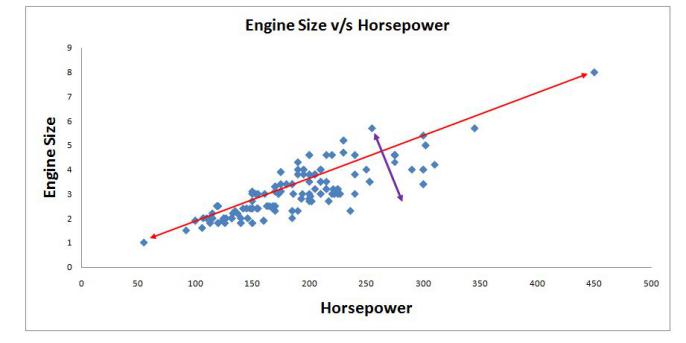
Note: How the extreme point on the right causes the variance to increase - this can be due to that data point being an outlier. This is the reason that outliers must be removed, or the data must be standardized, so that the effect of extreme values is curtailed.

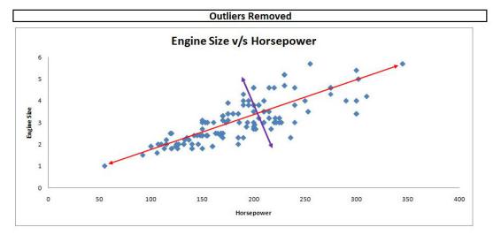
Now we bring this current situation to the earlier one, where we had variance on the X and Y axis - we have to rotate the graph so that these two lines become parallel to the X and Y axis, and this makes it easy to comprehend the variation in these lines. We can now draw the variance in terms of left and right as well as up and down. These two new rotated axes describing the variation in the data are known as Principal Components. Here the first Principal Component is the axis that has the most variation in the data (variation from left to right), while the second Principal Component has less variation (left to right). Thus from these two directions, we are able to quantify the most variation we have in the data.

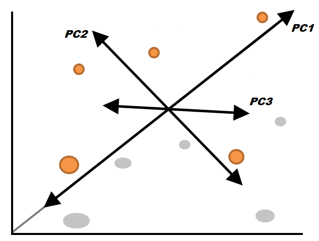
Now if we had three features in question, we would be having three directions, which basically means that we would be having three principal components, one for each variable. A similar process will follow for four, five, six, etc. variables, with Principal Component 1 spanning in the direction with most variation, Principal Component 2 spanning in the direction with the second most variation, and so on. Therefore, if we have 100 features, we will end up with 100 Principal Components. However, one must note that these axes are ranked in order of importance, with PC1 being the most important and PC2 being the second most important, and so forth.

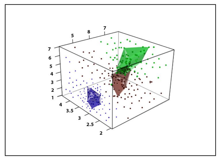
Thus in our data, if we have 64 variables, then there will be 64 dimensions, and we will end up with 64 Principal Components, but we want the data to be compressed into 2 dimensions, thus using information provided by two principal components. However, by using only two components, we lose a lot of information which would have otherwise helped us in classifying or predicting our target variable. Therefore, if we use only two components, thus compressing all our variables into 2 dimensions and projecting our target variable, our target variable will look very cluttered and will not be neatly separated; however, it will become easy for us to read such a graph. PCA, along with the loss of data, has other disadvantages also, such as it tends to find linear correlations between variables, which is sometimes undesirable.

Principal Component Analysis, despite its advantages and disadvantages, remains the most famous and widely used Dimensionality Reduction method, and should be used when dealing with datasets which are in very high dimensions.