Time Series in Python

Time Series models are used for forecasting values by analyzing the historical data listed in time order. This topic has been discussed in detail in the theory blog of Time Series. To demonstrate time series model in Python we will be using a dataset of passenger movement of an airline which is an inbuilt dataset found in R.

Preparation

Importing Preliminary Libraries

python

import pandas as pd
import numpy as np
import matplotlib.pylab as plt
%matplotlib inline
from matplotlib.pylab import rcParams
rcParams['figure.figsize'] = 15, 6
from datetime import datetime

Defining Format

For the date variable in our dataset, we define the format of the date so that the program is able to identify the Month variable of our dataset as a 'date'.

python

dateparse = lambda dates: datetime.strptime(dates, '%Y-%m')

Importing Dataset

We will import the above-mentioned dataset using pd.read_excel command.

python

time = pd.read_excel("C:/Users/user/Desktop/Data Sets/Time_Series/AirPassengersData.xls",parse_dates=['Month'],
index_col='Month',date_parser=dateparse)
time.head()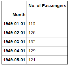

Indexing Data

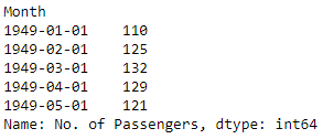
Instead of us using the name of the variable every time, we extract the feature of No. of Passengers.

python

time1 = time['No. of Passengers']
time1.head()

Graphical Representation

We will use the above-indexed dataset to plot graph.

python

time1.plot(kind="line",figsize=(10,5))

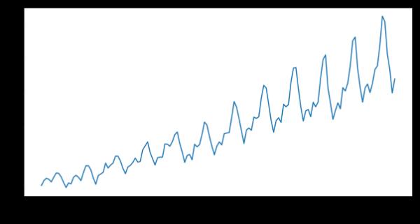
Air passengers line plot showing trend and seasonality

Clearly, there is a trend and seasonality graph. We will now look at different techniques for predicting the number of passengers for the next 10 years (By default Python, predicts values for ten years).

Averaging Techniques

There are mainly three types of averaging techniques - Simple Average, Moving Average and Weighted Average. These methods have been discussed in detail in the theory blog of Averaging Techniques. We will be demonstrating the Moving Average Technique and Weighted Average technique using Python.

Moving Average Technique

We can compute moving average using pd.rolling_mean function in Python. This will compute average using the data for the previous one year and plot the graph for the same.

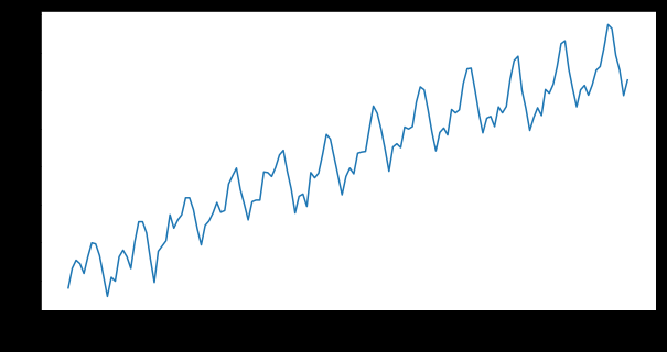
To compute the forecasted values we eliminate the trend using log transformation.

python

time_log = np.log(time1)
time_log.plot(kind="line",figsize=(10,5))

Log-transformed air passengers time series plot

Adding a Trendline.

python

moving_avg = time_log.rolling(12).mean()
time_log.plot(kind="line",figsize=(10,5))
moving_avg.plot(kind="line",figsize=(10,5),color='orange')

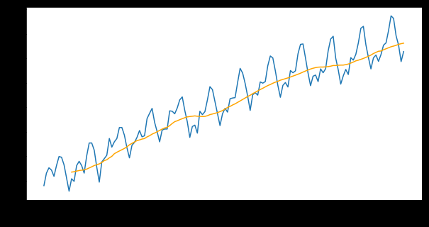
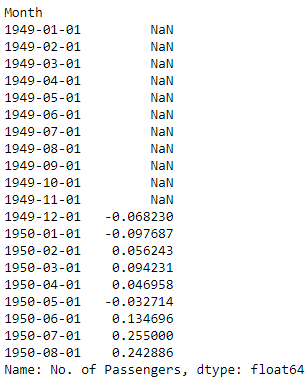
Log time series with moving average trendline

We can also compute the difference between the moving average and the log-transformed values.

python

time_log_moving_avg_diff = time_log - moving_avg
time_log_moving_avg_diff.head(20)

time_log_moving_avg_diff.head(20) output

Weighted Average Technique

Here the weights of the values are considered while computing the average value. The following code is used in Python to calculate weighted average mean and plot the graph for the same.

python

exp_wighted_avg = time_log.ewm(halflife=12).mean()
time_log.plot(kind="line",figsize=(10,5))
exp_wighted_avg.plot(kind="line",figsize=(10,5),color='orange')

We can also use the metrics command to calculate the error in our prediction.

python

time_log_ewma_diff = time_log - exp_wighted_avg
from sklearn import metrics
metrics.mean_squared_error(time_log,time_log_ewma_diff)

29.402106691858478

Note: this error is computed between time_log and the difference series time_log_ewma_diff (i.e. time_log − exp_wighted_avg), so the value is not a true forecast error against the smoothed series. It is shown here as in the original; for a genuine error, compare time_log with exp_wighted_avg after dropping the leading NaNs.

Smoothing Techniques

Various Smoothing Techniques have been discussed in the theory section. Here we will be using the techniques in Python to forecast values.

Seasonal Trend Decomposition

We will use seasonal_decompose package from statsmodels.tsa.seasonal for decomposition. This will deconstruct the time series into three components namely trend, seasonality and remainder. After getting the above-mentioned components we will plot the graph for them.

python

from statsmodels.tsa.seasonal import seasonal_decompose
decomposition = seasonal_decompose(time_log)
trend = decomposition.trend
seasonal = decomposition.seasonal
residual = decomposition.resid
plt.subplot(411)
time_log.plot(kind="line",figsize=(10,6),label='Original')
plt.subplot(412)
trend.plot(kind="line",figsize=(10,6),label='trend')
plt.legend(loc='best')
plt.subplot(413)
seasonal.plot(kind="line",figsize=(10,6),label='Seasonality')
plt.legend(loc='best')
plt.subplot(414)
residual.plot(kind="line",figsize=(10,6),label='Residuals')
plt.legend(loc='best')
plt.tight_layout()

Seasonal decomposition 4-panel plot showing original, trend, seasonality, and residuals

From the above graph, we can find the number of 'seasonal periods' and use that value for Exponential Smoothing.

Exponential Smoothing Method

There are mainly two types of Exponential Smoothing Methods - Simple Exponential and Exponential Smoothing aka Holt Winter Method. These have been discussed in detail in the theory blog of Smoothing Techniques. Both these techniques will now be demonstrated in Python.

Simple Exponential Smoothing Method

This method is used for forecasting when there is no trend or seasonal pattern.

Importing Libraries

We will import Exponential and Simple Exponential Smoothing library from statsmodels.tsa.api package.

python

from statsmodels.tsa.api import ExponentialSmoothing, SimpleExpSmoothing, Holt

Conducting Simple Exponential Method

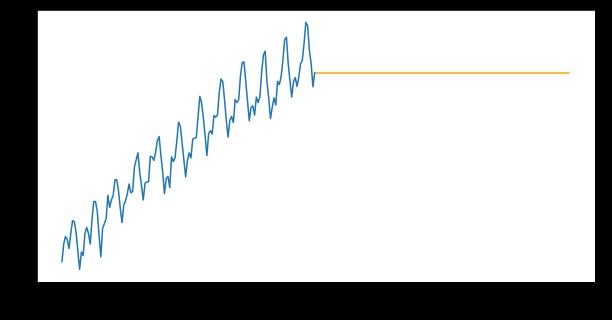
We will now run the code for Simple Exponential Smoothing (SES) and forecast the values using forecast attribute of SES model.

python

ses = SimpleExpSmoothing(time_log).fit(smoothing_level=0.6,optimized=False)
ses1 = ses.forecast(len(time_log))

Plotting Graph

We now plot a graph from the above output.

python

time_log.plot(kind="line",figsize=(10,5))
ses1.plot(kind="line",figsize=(10,5),color='orange')

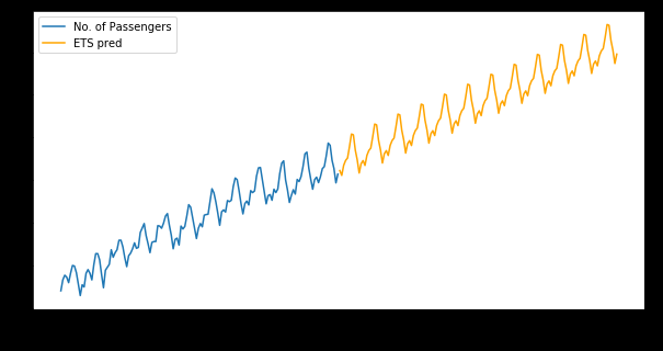
Simple Exponential Smoothing forecast plot

Exponential Smoothing Technique (EST) aka Holt-Winters Method

The Exponential smoothing technique assigns less weight (importance) as the observations get older and have been discussed in the theory section.

Running the Code for EST

We first run an ETS model using ExponentialSmoothing.

python

ets_stl = ExponentialSmoothing((time_log) ,seasonal_periods=12 ,trend='add',
seasonal='add').fit()
ets_stl1 = ets_stl.forecast(len(time_log))

Plotting Graph

We then plot a graph from the above output.

python

time_log.plot(kind="line",figsize=(10,5),legend=True)
ets_stl1.plot(kind="line",figsize=(10,5),color='orange',legend=True,label='ETS pred')

Holt-Winters Exponential Smoothing forecast plot

ARIMA Models

ARIMA Models have been explored in the theory section. Here an automated way of forecasting is performed by using ARIMA models.

We will import ARIMA from statsmodels.tsa.arima_model library.

python

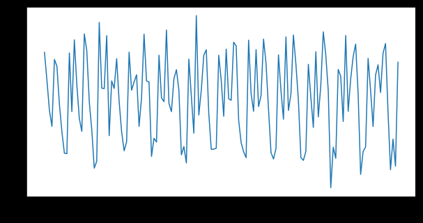
from statsmodels.tsa.arima.model import ARIMA
time_log_diff = time_log - time_log.shift()
time_log_diff.plot(kind="line",figsize=(10,5))

python

model_ARIMA = ARIMA(time_log, order=(2,1,2))
results_AR = model_ARIMA.fit()
time_log_diff.plot(kind="line",figsize=(10,5),title=('MSE: %.4f'%
metrics.mean_squared_error(time_log_diff,results_AR.fittedvalues)),
label='time_log_diff',legend=True)
results_AR.fittedvalues.plot(kind="line",figsize=(10,5),color='orange',label=
'ARIMA Results',legend=True)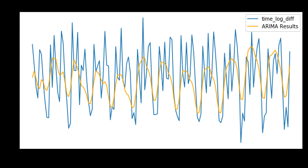

ARIMA fitted values vs actual differenced series

In this blog post, many of the forecasting techniques were explored. The same techniques have also been explored in the blog Time Series in R.