// descriptive statistics

Measures of Central Tendency

Measures of Central Tendency is another majorly used Descriptive statistic. Measures of Central Tendency try to summarise the data by a single value that represents the middle of the distribution. There are three Measures of Central Tendency: Mean, Median and Mode.

Mean

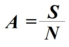
Mean is the arithmetic average of a distribution of scores. It provides a rough summary of the distribution; however, it does not tell anything about the spread of the distribution. Mean can be calculated by taking the sum of all the observations in a dataset and dividing it by the number of observations, i.e.

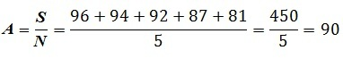
For example, there is a dataset with 5 values: 96, 94, 92, 87, 81. We can calculate the mean of this dataset by adding all the values (S = 450) and dividing it by the number of observations (N = 5).

Worked example: the mean of 96, 94, 92, 87 and 81 is 450 divided by 5, which equals 90 — The arithmetic mean of this dataset is 90.

There are certain advantages and disadvantages with mean. While the mean can provide a quick summary of a dataset and can be used for continuous as well as discrete datasets, it cannot be used for qualitative data (Categorical variables). Also, mean is highly sensitive to extreme values and can provide a very biased outcome if there are outliers in the data. Also, the shape of the distribution can influence the outcome of mean and, especially if the distribution is skewed, the mean can provide misleading results. Mean also fails in explaining the spread of the scores (variance) and the number of scores in a distribution close to the mean.

In the introduction of this section, the difference between a parameter and a statistic was explained. When mean is calculated from a population dataset then the mean is a parameter denoted by the symbol μ; however, if mean is calculated from a subset of this population, i.e. from a sample, then the calculated mean is a statistic denoted by the symbol x̄. Therefore the formula for calculating Population mean will be μ = ( Σ X_i ) / N, while the formula for calculating Sample Mean will be x̄ = ( Σ x_i ) / n, where x̄ is the sample mean, μ is the population mean, Σ means "the sum of", X is an individual score in the population distribution, x is an individual score in the sample distribution, n is the number of scores in the sample, and N is the number of scores in the population.

Median

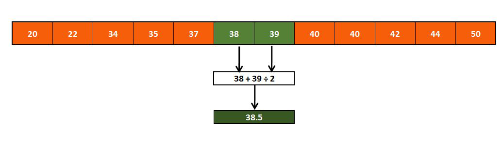
Median of a given dataset can be found when the values of the dataset are arranged in ascending or descending order and the middle value, or the value that marks the 50th percentile of this dataset's distribution, is called its Median. The Median divides and distributes the dataset into two equal halves with 50% of observations on each side.

However, if the number of values is even, then in that case we have to calculate the median by taking an average of the middle two values.

An even number of sorted values with the two middle values averaged to give the median — With an even count, the median is the average of the middle two values.

There are certain advantages that median has over mean, and the main ones are that median doesn't get affected by outliers or if the distribution of data is skewed. Median, however, cannot be used for certain types of categorical data such as Nominal Categorical Data, as they cannot be ordered on the basis of their weights since the values do not have any weight and cannot be ordered logically.

The Mean and Median are the measures of Central Tendency that are some of the most useful statistics as they provide information about the whole distribution in a single number; however, it is very important to note that they ignore a great deal of information about the distribution, making it easy for them to be misused and to make sweeping generalisations based on mean or median.

Mode

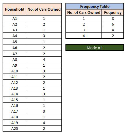
Mode can be calculated by calculating the occurrence of scores in a distribution. It is among the least used Measures of Central Tendency because it does not provide much information. For example, there is a dataset having the number of cars owned by a household. In the below example, we surveyed 20 houses and the mode is the number that gets repeated the most often.

Mode is more useful than mean or median in the sense that it can be used for both numerical as well as categorical data, but suffers when there are no repetitions among the values (Continuous Numerical Data) or if there is more than one mode in a distribution (Bi-Modal or Multi-Modal Distributions). Under such circumstances the descriptive capabilities of mode get limited.

Outliers and Measures of Central Tendency

In all three Measures of Central Tendency, it is mentioned how they may or may not be vulnerable to outliers. Here we explore this with examples explaining how Mean, Median and Mode may or may not get affected by Outliers.

Outliers and Mean

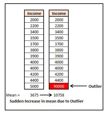
A dataset where adding one very large outlier sharply increases the mean — A sudden increase in the mean due to an outlier.

Here it is very evident how, due to one unproportional value, the mean gets affected. Thus, if in a dataset there are values that are too large or too small compared to the rest of the values, then it can cause the mean to deviate.

Outliers and Median

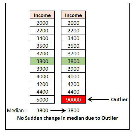
The same dataset with an outlier, where the median stays unchanged — No sudden change in the median due to the outlier.

We can see how median is not affected by the outlier, as when the data is sorted, the outlier either ends up at the beginning (if the outlier is very small in weight) or at the end (if the value of the outlier is too large), and the middle value remains intact.

Outliers and Mode

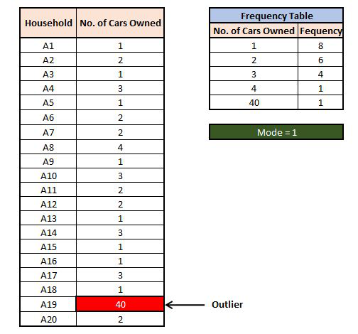
The mode example with an outlier added, where the mode stays unchanged — We add an outlier to the earlier example for mode and find that mode too does not get affected by outliers.

Therefore, among all the Measures of Central Tendency, mean is the most vulnerable to outliers while the others are less vulnerable to them.

Thus Measures of Central Tendency help us in understanding our data by providing us with one value. Various Measures of Central Tendency can be used, with Mean being used for numerical and the Mode being used for categorical data. However, they all fail to explain the distribution of data: for example, a variable having the value 6 for six times will have a mean of 6, and a variable having values 2, 3, 4, 6, 8 and 13 will also have a mean of six. Therefore it becomes very important to understand the distribution of the data, and this leads us to Measures of Variability, using which we can understand the spread of the data.