// f tests

One Way ANOVA

One way ANOVA is used to compare means of the groups of an independent variable to see if the groups are significantly different from each other or not. It is important to note that the independent T-Test can also be used if the independent variable has only 2 levels (groups). Here the only difference between the T-Test and One Way ANOVA will be that T-Test will produce a T value while ANOVA will produce an F Ratio which is nothing but the T value squared, still, the results will be identical. However, T-Test cannot be used if the levels in the independent variable are more than two. For example if we have an independent variable with three levels - X, Y and Z then we have to run three separate T-Tests comparing X with Y, Y with Z and Z with X and each time we run a test i.e. the more times we run the T-test, the chances of making a Type I error will increase.

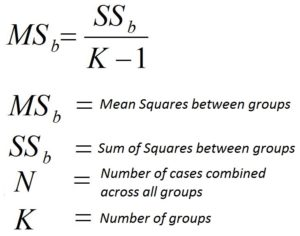
Coming back to One-way Analysis of Variance, the purpose of it is to test whether group means are equal or not. For this, we calculate an F ratio for which we divide the variance of the independent variable into two components: variation between sample means and variation within the samples i.e. variance attributable to between-group differences and variance attributable to within-group differences. Thus in One-Way ANOVA, the F-statistic is the following ratio: F = variation between sample means ÷ variation within the samples.

Intro to F Ratio

Before getting into the details of how we calculate the F Ratio, we must understand why we divide the variation between the groups with the variation among the groups. To understand this, we use an example.

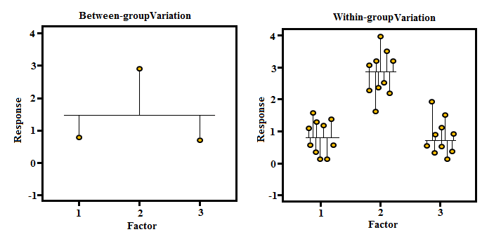
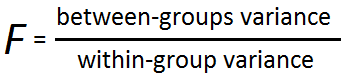
Imagine you are an owner of a clothing store and launch a Christmas offer where you decide to pick 1,000 of your customers randomly and categorise these customers into 3 groups. The Group I will be who have spent on average Rs. 10,000 on your store and will be offered a gift card worth of Rs. 1,000. Similarly, the Group II and III will be who have spent Rs. 5,000 and Rs. 1,000 in your store and will be offered a gift card worth of Rs. 500 and Rs. 100 respectively. Now before going ahead with the offer you want to make sure that the groups are meaningful and thus require to know if these groups are actually (statistically) different from each other. You analyze the first group and it turns out that the customers in the first group have spent something like this- 20000, 6000, 12000, 4000, 8000 etc. Here if we see closely then the average will be 10,000 only (20000 + 6000 + 12000 + 4000 + 8000 ÷ 5 = 10,000), however, the value varies a lot and thus the groups are not meaningful but if the sample had the values such as 10000, 9000, 13000, 8000, 10000 then the group would have made much more sense as the variation within the group would have been less. However for this Group I to remain different from the Group II, the variation between the groups should be high. Thus to state that the difference between the groups is significant, the variance within the groups should be low however the variance between the groups should be high and this leads us to the formula of the F-statistic used in the One way Analysis of Variance which is this ratio of variation between sample means and variation within the samples.

Calculation- the formula for finding the F ratio in statistical terms is F = MS_b ÷ MS_e, that basically means F = between-groups variance ÷ within-group variance.

Here the Numerator is the Mean Square between the group (what we have been calling- finding the variance between the groups) and the Denominator is the Mean Square Error also known as the Mean Square Error within groups (what we have been calling- finding the variance within the groups). ANOVA finds if the average amount of difference (variance) found between the groups is large or small when compared to the average amount of difference (variance) found within the groups. Thus the process to find the F Ratio includes-

Step 1- Finding the average variation between each of our sample groups (levels)- Mean Square Between (MSb).
Step 2- Finding the average variation within each of our sample groups (levels)- Mean Square Error Within (MSwithin) also known as Mean Square Error (MSe).
Step 3- Once MSb and MSe are found, divide them to get the F value.

Calculating MSb (Mean Square between) (Numerator of F Ratio)

Unlike the numerator of T value which simply finds the difference between the two means, ANOVA requires finding the average difference between the means because there can be more than two groups (levels) within an independent variable and thus it requires to find the average of the difference of sample means. The formula to find the MSb is SSb divided by degrees of freedom for the SSb-

Finding the Numerator of MSb (SSb)- SSb is the sum of square between the groups which can be calculated by:

Step 1- Subtract the Grand mean (Mean of the independent variable) with the group mean.
Step 2- Square each of these deviation scores.
Step 3- Multiply each squared deviation by the number of cases in each group.
Step 4- Add these squared deviations from each group together.

Example- We have an independent variable A with levels (groups) X, Y and Z:

Step 1: Find the mean of the variable A and the mean of groups X, Y and Z.
Step 2: Subtract the group mean with the grand mean and square it.
Step 3: Do the above step for each case in the group.
Step 4: Add all the values.

e.g. - (4−8)² + (4−8)² + (4−8)² + (8−8)² + (8−8)² + (8−8)² + (12−8)² + (12−8)² + (12−8)² = 96.

Here our SSb comes out to be 96.

Finding the Denominator of MSb (degrees of freedom of SSb)- to find the degrees of freedom for SSb we subtract the number of groups (levels) in the independent variables by 1 (K-1 where K is the number of levels in an independent variable).

Now as we have the numerator and the denominator for MSb, we simply divide the SSb with its degrees of freedom i.e. 96 ÷ (3−1) = 48. Thus here our MSb comes out to be 48.

We must remember that the MSb indicates the variance between the groups and as per the example (Christmas offer example) we want the variance to be high which suggests that the Group I, II and III are different from each other and for this group means should not be clustered close to the overall mean because if they do then it will mean that their variance is low. However, if the group means are spread out further from the overall mean (mean of the independent variable) then it will mean that the variance between the groups is higher.

Calculating Mean Square Error Within (MSe or MSwithin) (Denominator of F Ratio)

We can measure how much the group means are different from the independent variable mean but as mentioned in one of the above examples, each group or level should have less variance if we want to carry on with our Christmas offer. For this, we need to calculate how far each observation is from its group mean for all the observations. Unlike the difference between the numerator of t value and f value, the denominator of the fraction for T-Test and the denominator of the F value (which is the Mean Square Error within) is almost identical as in T-Test, the denominator indicates the standard error of the difference between the two sample means and here the MSe (denominator of F value) means the square of the average error within the groups (i.e. the average variations within the group).

Finding the Numerator of MSe (SSe)- SSe is the sum of square error within the groups which can be calculated by:

Step 1- Subtract the Group mean by individual score.
Step 2- Square the above-calculated value.
Step 3- Add all such values.
Step 4- Do this for all the groups and add them all to come up with one final number.

Example- have an independent variable A with levels (groups) X, Y and Z (same data as above):

Step 1: Find the mean of the variable A and the mean of groups X, Y and Z.
Step 2: Subtract the value of a group with its group mean and square it.
Step 3: Do the above step for each case in the group.
Step 4: Add all the values.

e.g. - (6−4)² + (4−4)² + (2−4)² + (6−8)² + (10−8)² + (8−8)² + (10−12)² + (12−12)² + (14−12)² = 24.

Finding the Denominator of MSe (degrees of freedom of SSe)- the degrees of freedom for SSe can be found by taking the number of values within each group and subtracting 1 from each group or to put it simply it is N-K where N is the Total number of cases for all groups and K is the total number of groups. (Notice how this is almost identical to the formula of degrees of freedom used for the independent sample T-Test.)

Now as we have the numerator and the denominator for MSe, we simply divide the SSe with its degrees of freedom i.e. 24 ÷ (9−3) = 4.

SSb v/s SSe

SSe subtracts the group mean from the individual score in each group while SSb subtracts the grand mean (independent variable’s mean) from each of the group’s mean. SSb multiplies each squared deviation by the number of cases in each group and it provides us with the approximate deviation between the group mean and the grand mean for each case in every group while SSe subtracts the Group mean by the individual score, squares it and adds them after doing this for all the groups.

SSb degrees of freedom v/s SSe degrees of freedom

K is the number of groups and N is the total number of samples in the independent variable. To convert SSb to MSb we require the SSb to be divided by its degrees of freedom which here is K-1 (df=K-1). On the other hand if we have to convert SSe into MSe, we have to divide SSe by its degree of freedom (which here is number of samples in each group with each of them subtracted by 1) and after doing this for all groups, we have to add them up ((n1−1) + (n2−1) + (n3−1)…) or we can simply subtract the Total number of groups from the Total number of Samples (N-K).

SSb + SSe = Sum of Squares Total (SSt)

If we add SSb and SSe, we end up with the sum of squares total (SSt) which is total variance in the entire dataset. To understand this, we can use another example using the same independent variable A with levels (groups) X, Y and Z.

Step 1: Find the mean of the variable A and the mean of groups X, Y and Z.
Step 2: Subtract the value of each group with the grand mean (mean of the independent variable).
Step 3: Square the output from the above step (to remove the negative).
Step 4: Do the above step for each case in the group.
Step 5: Add all the values.

e.g. - (6−8)² + (4−8)² + (2−8)² + (6−8)² + (10−8)² + (8−8)² + (10−8)² + (12−8)² + (14−8)² = 120.

Interestingly the SSb and SSe that came out using this dataset was 96 and 24 respectively and if we add them the output is 120 which is our SSt.

Calculating F Ratio

Here the F-statistic is the ratio of variation Between Sample Means and Variation Within the Samples and their values are expected to be roughly equal under the null hypothesis (i.e. that the groups are same and have equal mean) producing an F-statistic which is approximately 1. F Ratio is very useful as it includes both the variations discussed in the above sections. If the F value is high then it means that the variability of group means is large relatively as compared to the within-group variability.

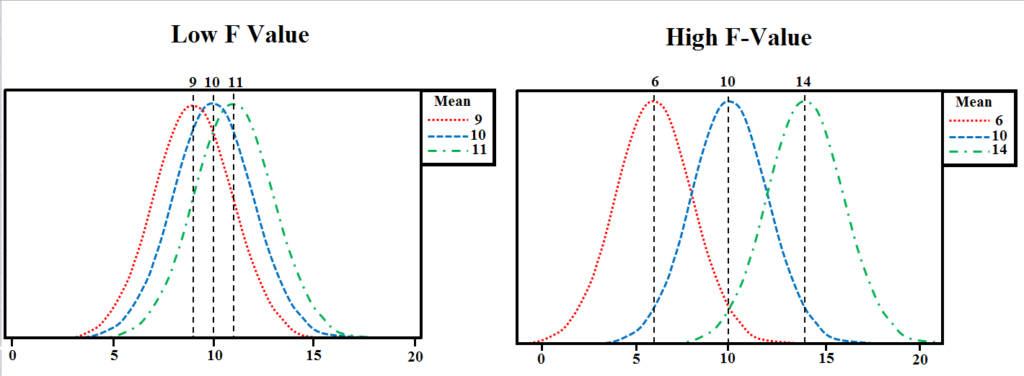
On the other hand, if the F value is small i.e. close to 1, it means that the variability among the groups is low and within the group is high. If we have to reject the null hypothesis which states that the group means are equal, we need a high F-value (Unlike the P value where if the P value is high compared to our significance level which is generally set at 0.05, the Null Hypothesis is accepted). In the above example, the F Ratio comes out to be 12 (MSb ÷ MSe = 48 ÷ 4).

But the question is, how high an F-value should be to reject the null hypothesis and for this is what has been discussed in the below section.

Using F Statistic for Hypothesis Testing

When the Null Hypothesis is true i.e. the means of the groups are equal to each other, the F statistic (which is the ratio of the variance among the group and variance within the group) follows an F-Distribution.

To know how statistically significant the change in the means of the group is, we have to place our F value on the F Distribution to see if our result lies in the critical region of the F Distribution. Note that the higher our F value is, the more evidence we have against the Null Hypothesis. Now we require to calculate the probability of having such an F value by chance and to know the probability we place our F value on the F Distribution (when the Null Hypothesis is true, F statistic has an F Distribution) and this F distribution is based on the number of degrees of freedom we had in the numerator and the denominator of the F Ratio.

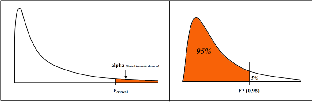
Now when we plot our F statistic, the probability of getting such an F value by chance i.e. getting such an F value or a value greater than this is the area under the curve (i.e. area to the right of our F value). So the probability of getting our F value or something farther out in the right tail is the area under the curve. We look at our F table to find the area to the right of our F value. We have to consider the degree of freedom we had in the numerator and the denominator and look at the various p values provided to us and find the area to the right of the curve for various significance level (α).

Here the tables may not provide a very accurate answer and statistical software can be used to find the exact p-value and if the p-value is greater than our significance level then we accept the Null otherwise if the p-value is lower than our significance level, we reject the Null Hypothesis and are able to say that our F value is high enough to reject the Null Hypothesis.

Assumptions for One Way ANOVA

We assume that the population is normally distributed and the samples are independent. The sample size and variation in each group are roughly the same.

Effect Size

It is important to note a thing about statistical significance which has been mentioned earlier also that a very strong statistical significance, doesn’t automatically indicate that the results are practically significant as when the sample size is very large, even a small difference can be calculated by the test as a statistically significant difference which in real life application may not be considered as a serious change. So it is important to keep the practical interests in mind.

Post Hoc Test

One of the problems with One Way ANOVA is that it doesn’t tell us which groups differ from each other significantly and which don’t. For this a Post Hoc test can be conducted. There are many kinds of Post Hoc Tests such as-

• Tukey’s HSD Test (HSD: Honestly Significantly Different)
• Duncan’s new multiple range test (MRT)
• Dunn’s Multiple Comparison Test
• Holm-Bonferroni Procedure
• Bonferroni Procedure
• Rodger’s Method
• Scheffé’s Method

Some of these tests are more conservative than the other i.e. makes it difficult to have statistically significantly different groups but they all follow the same principles where each group’s mean is compared with the other and is determined if they are significant from each other or not.

A Priori Contrasts

A Priori Contrasts are used when we want to know the particular groups or the combination of groups that are different from each other in their mean averages on the dependent variable. An example can be of an Independent Variable where there are 4 groups - A, B, X and Y and want to know if A and B are statistically different from X and Y. These things can be used by A Priori Contrasts.

One-way ANOVA helps us in comparing the various groups of an independent variable. However, there are situations when there is more than one independent variable and this brings us to our next topic, Factorial ANOVA.