// inferential statistics

T Tests

T-Tests are a type of hypothesis tests. An introduction to them was given in Brief Introduction to T-Tests. T-Tests are used when we have to compare two means and have to determine if they are statistically different from each other or not. T-Tests use the family of T Distribution and T table is used to find the p-value. As explained in earlier blogs related to T-Tests and Hypothesis Testing, T-Tests are used when the sample size is less than 30 (small sample size) or the standard deviation of the population is not known.

There are mainly three types of T Tests:

• One-Sample T-Test
• Paired two sample T-Test (Dependent T-Test)
• Independent two-sample T-Test (Independent T-Test)

One-Sample T-Test

One sample T-Test is the most basic type of all the T-Tests and perhaps also the most crucial one as it can be used to explain how all the T-Test work. One-Sample T-Test is generally used when we have to find if our sample mean is equal to the population mean or is significantly different i.e. when we have to compare one sample mean to a null hypothesis value. To conduct this T-Test, one categorical independent variable and one continuous (interval scaled) dependent variable is required. T-Test requires us to follow steps similar to any other hypothesis test where first, a value has to be found which here will be the T-value, and based on this T value along with degrees of freedom, we can find the p-value by looking into the T Table to determine if the Null Hypothesis is to be rejected or not. The Null Hypothesis is that there is no difference between the Sample Mean and the Null Hypothesis value (e.g. the population mean) i.e. H0: u1 = x1. The alternative hypothesis, however, is that the two values are statistically significantly different from each other i.e. HA: u1 ≠ x1. The assumption here is that the variables are approximately normally distributed.

To understand how One sample T-Test works, it is important to understand how the T value is calculated. The formula for T Value is-

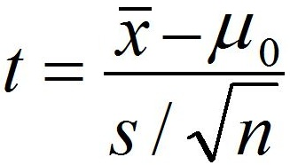
One of the most common and easy way to understand the formula for T-Test is by using the analogy that T value is like the signal-to-noise ratio where the numerator is the signal and the denominator is the noise.

The numerator which is the value calculated after subtracting the sample mean from the Null Hypothesis value say the population mean can be considered as the Signal of the Signal-to-noise ratio and as the difference between the sample mean and the null hypothesis value increases (in either of the direction i.e. the output can be a negative or a positive number), the output also increases and consequently the ‘strength’ of the signal increases and on the contrary if the strength of the signal is very weak say 0 (if there is no difference in the sample mean and population mean producing 0 as a result), the entire ratio will be a 0.

The denominator of the formula for t value is standard error of mean and as discussed in the blog Standard Error, Standard Error of Mean and Central Limit Theorem, the standard error of mean indicates how close our sample mean is to the mean of the population, thus higher the value of the denominator, less precise it is in determining the mean of the population (higher value mean more random error). Here the denominator is analogous to Noise in the sense that as the noise increases, the difference between the sample mean and the null hypothesis value increases and thus the noise is included in the fraction so as to determine if the signal is large enough to be considered significant.

Thus signal to noise ratio (T value) indicates how distinguishable the signal is from the noise so if the signal is not large enough or the noise is too large causing the signal not to stand out and consequently producing a low ratio (low T Value), then the null hypothesis is to be considered (after considering the p-value and significance level) and it is to be concluded that the difference between the sample mean and population mean is being observed due to random chance.

Note that Degrees of Freedom are also to be considered. The degrees of freedom are calculated by subtracting 1 from N (number of samples) and once the t value and degrees of freedom are available, T table can be used to find the p-value to reject or accept the null hypothesis.

Paired two sample T-Test (Dependent T-Test)

One-Sample T-Test and Paired two sample T-Test are almost one and the same thing. Here unlike One-Sample T-Test (where the sample mean is compared with the Null Hypothesis value), two means on a single sample or of two matched/paired samples are compared (e.g. before and after). Note here the levels of the variable can be attributed to time (before and after) which is very similar to Repeated Measures ANOVA, however, the assumption for normality are slightly different in both of them as Paired Dependent T-Test requires the continuous variable to be approximately normal while Repeated measures ANOVA require each level (group) of the continuous variable to be normal.

One Sample and Paired Two sample work in a similar manner, as paired sample T-Test simply calculates the difference between paired observations (e.g., before and after) and then on the differences, 1-sample t-test is performed.

The paired t-test has some advantages as it can work if the assumption of normality is violated, however, the distribution should be continuous, unimodal (having only one mode) and symmetric. If the distribution is not even approximately close to a normal distribution then nonparametric procedures are to be used.

A quick way to decide if One sample T-Test is to be used or any other T-Test is to see if the ‘before and after’ scores in each row of the dataset represents the same subject. (A row in a dataset shows marks of student ‘A’ before academic coaching and after coaching, here as the subject is same, Paired two sample T-Test can be used). However, if the difference in the values doesn’t belong to the same subject then Independent two-sample T-Test is to be used.

Example of Dependent t Test can be- Is there a change in the average marks obtained by a group of students on a standardised test? They took two exams- one exam at the beginning of the academic year and another one at the end of it.

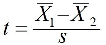
Thus for this example, the formula used for calculating the t value in Paired two sample T-Test will be-

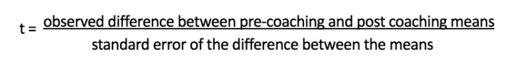
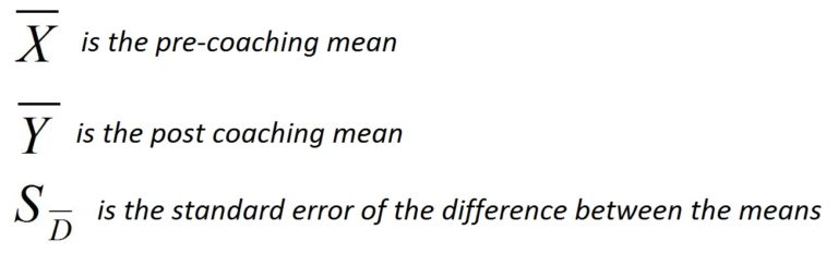
or

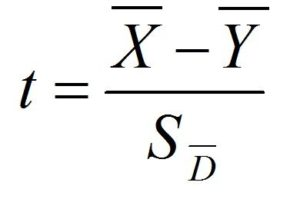
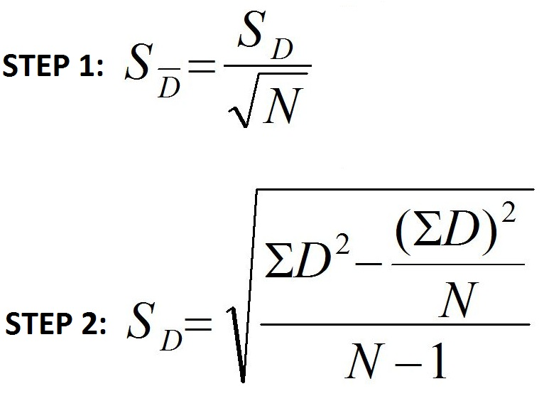
Here as the difference (between the two scores of each student) will sometimes be positive, sometimes negative and sometimes it will be null (no improvement in marks), and these values will form their own distribution with a mean and standard deviation, and this standard deviation will be the standard error of the difference between the means (samples) and is used as the denominator in the fraction to calculate the t value. The two-step formula to calculate this standard error of the difference between dependent sample means is-

Once the t value is calculated, we require degrees of freedom to find the p-value from the T table and the degrees of freedom for Paired two sample T-Test can be calculated by subtracting 1 from the number of pair of scores (marks).

Independent Two-Sample T-Test

Independent Two-Sample T-Test is used when we have to compare means of two independent samples of a variable and is very similar to one sample T-Test but to conduct such a T-Test, independent groups for each sample are required. Also, we require one categorical (nominal) independent variable which has two levels (subcategories/groups) and one continuous (interval scaled) dependent variable. Example of such a problem can be of finding if the height of men and women is different from each other or not, thus the two sample T-Test is used to find if the mean of the two samples are statistically significantly different from each other or not i.e. if the difference is large enough to allow us to draw an inference about the population they represent or the difference is just due to random sampling and the result can be different or even be opposite in another sample. Thus finding the standard error is crucial and the analogy used above (signal and noise ratio) can be used when it comes to understanding the formula used to calculate the t value for Independent Two-Sample T-Test. The formula to calculate the T value is-

Here the numerator is the difference between the means of the two samples (signal). The denominator (noise) is the standard error. The standard error here unlike the one in One sample T-Test is not the sampling error of mean but is the standard error of the difference between Independent Sample Means and requires to combine standard deviations of the two samples. However, it is not that simple as we can either assume that the variability in both groups is equal or is not equal. If we assume that the variance in each sample is about equal and if sample size of the two means is same or is approximately the same then if we combine the standard deviation of the two samples, the output comes out to be the Standard Error of the difference between the means (denominator of the T value formula).

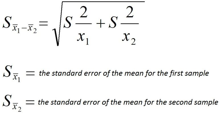
However, if the sample size is not the same then the formula needs to be adjusted/modified. This happens because when we assume that variance in each sample is same and assign equal weight to each sample then little variance creates a very large standard error if the two sample sizes are not ‘almost equal’. When the variances or the sample sizes are unequal, Welch's t-test (the unequal-variances t-test) is used, which adjusts the formula and the degrees of freedom. The standard error of the difference combines the two variances as the square root of (s1^2/n1 + s2^2/n2), not by simply adding the two standard deviations of the samples.

Once the T value is found, the T chart can be referred to find the p-value, however, before that we need to find the degrees of freedom which in this T-Test is to take the sum of the sample size of the two samples and subtracting two from it i.e. df = N1 + N2 − 2 (N1 = sample size of sample 1 and N2 = sample size of sample 2). The degrees of freedom are important as the shape of t distribution changes and so do the probabilities associated with it. Thus we use the degrees of freedom which is a function of the size of the samples.

Here also, the null hypothesis is that the two population means are equal while the alternative hypothesis states otherwise (equal variance is an assumption of the test, checked separately, not the hypothesis being tested). Also, here the signal to the noise principle applies where if the signal stands out then we can reject the null hypothesis. To have a precise result we have to determine the significance level. We refer the T-Test table to find the p-value for the corresponding t value and degrees of freedom and if the p-value is less than the predetermined significance level then the null hypothesis can be rejected and the two means of the sample can be said to be statistically significantly different from each other.

The three types of T-Test explored in this blog play a major role in inferential statistics. They can be used when we don’t have a large enough sample size or the standard deviation of the population is missing and this is the reason they are so popular as they act as an alternative to Z Tests.