// feature engineering

Feature Transformation

Feature Transformation means the replacement of a variable by a function, as it often helps to transform complex relationships which can be non-linear into linear relationships, and also helps in transforming distributions that are not normal into a normal distribution. Various methods of transformation can be used to achieve the above-mentioned results.

Scenarios for Using Transformations

Non-Linear Relationships

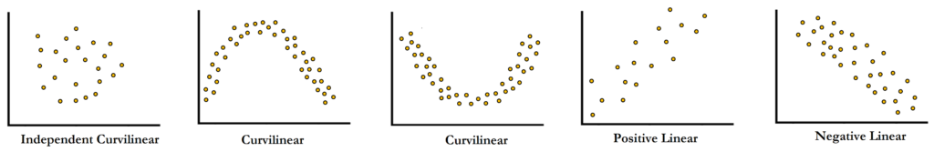
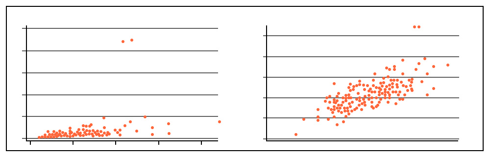
If we use a scatterplot to see the relationship between two continuous variables and find that they do not share a linear relationship, then transformations are often used, as it is a process that changes the distribution or relationship of a variable with others, often improving predictions. Log transformations are among the most common transformations used here. A typical example where such transformations are required is when handling Sales and Income data.

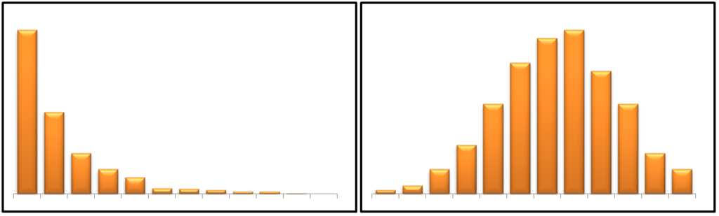
Skewed Data

Data can be skewed due to various reasons, such as extreme outliers (as discussed in Measures of Shape). The skewness of data can cause problems, as for a lot of parametric statistical tests the underlying assumption is that the data is normally distributed, and feature transformation, such as by using log transformations, can make a very skewed distribution shift a bit towards a normal distribution, consequently making the data fit the assumptions better. This can help in detecting patterns in the data. Distributions which are positively skewed can be made to conform more closely to the normal distribution by using square/cube root or log transformations, while negatively skewed distributions can be made to conform more closely to a normal distribution by taking the square/cube or exponential of the variable. For example, the log transformation is widely used in biological, biomedical and psycho-social research to deal with skewed data, as many biological variables do not meet assumptions such as being normally distributed or having homogeneous standard deviations, which are required for various parametric statistical tests. Transformations also help in controlling the effect of outliers and can be used to treat outliers.

Methods of Feature Transformation

As hinted above, there are various methods of feature transformation, each having its own strengths and scenarios where it can be put to best use. These transformations refer to the replacement of a variable by a function, such as replacing a variable ‘Sales’ by its logarithm or square/cube root. The various transformation methods are listed below.

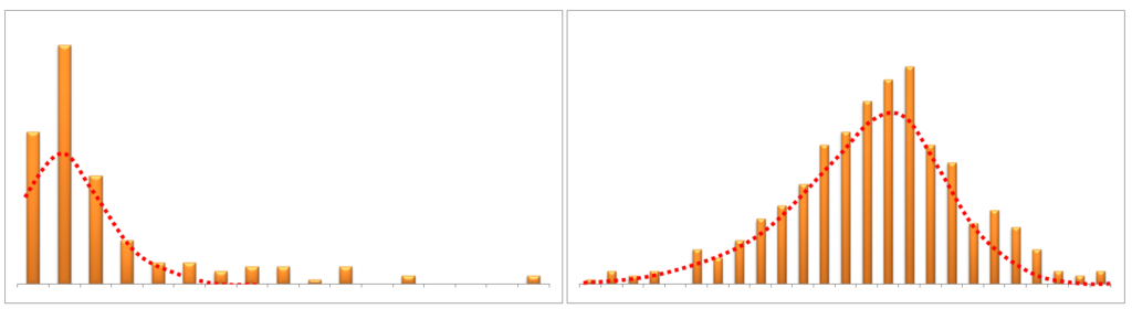
Logarithm

It is one of the most common methods of transformation, where the process consists of taking the natural logarithm of the variable, with the log of each observation taken, generally reducing the skewness of the variable. Mathematically, if we multiply various independent variables together, then the output is log-normal. Data belonging to certain domains is highly responsive to log transformations, such as when dealing with biological variables, which are generally skewed; log transformation helps in making the distributions normal, often exposing hidden patterns in otherwise cluttered data. Log transformations can also be used if the data’s relationship is close to exponential.

However, one must note that log transformations cannot be applied to zero or negative values, and a constant is required to be added to each number to make them positive and non-zero.

Square / Cube Root

Although transforming a feature by the use of square or cube root is not as popular or significant as logarithmic transformation, it can be used, such as when a variable is a count of something. The process of this transformation consists of taking the square root of each observation, and as we take a square root of the values, it can be applied to even negative values including zero, unlike log.

Arcsine Transformation

Also known as the arcsine square root transformation (or the angular transformation), it consists of taking the arcsine of the square root of a number. In some cases, two times the arcsine of the square root of a proportion is calculated, making the arcsine scale go from zero to pi; however, if it is not multiplied by two (Sokal and Rohlf 1995), the scale stops at pi/2. This choice is generally arbitrary. The output is in radians and can range from 0 to π/2. Variables that range between 0 and 1 can be transformed using arcsine transformation, and thus such a transformation is used for proportions.

Feature Transformation methods provide us with a quick and easy way of making the data fit for various kinds of modeling algorithms. Transformations are particularly useful when the distribution of the data is not normal. Various kinds of Feature Transformation methods have been explored above and can be used depending upon the type of data.