// miscellaneous methods

Outlier Treatment

Outlier treatment is another important step in data pre-processing and can be performed before missing value imputation (one may prefer doing missing value treatment once outliers are treated, especially if using mean imputation, as outliers can skew the data). An outlier as such is an observation that lies an abnormal distance from other values, or any observation far away from the mass of data or the overall pattern. Outliers can be mild and extreme, with the extreme being away from the source by a great deal. Also, an outlier can be looked for in each variable (Univariate Outlier) or can be looked for in relation to other variables (Bivariate Outlier).

As discussed in Measures of Central Tendency and Measures of Variability, an outlier can adversely and significantly affect various statistics, with certain statistical and machine learning models being very vulnerable to outliers. Outliers can be caused due to various reasons such as incorrect or inefficient data gathering, data entry errors such as a human error made during entering the data in a spreadsheet, industrial machine malfunctions where the machine malfunctions eventually reflecting wrong values in the output data, measurement errors where the data supposed to be in a particular measurement unit (e.g. Kg) is presented in a different measurement unit (e.g. grams), sampling errors where samples are taken from a population which is not in question (such as while gathering income of school teachers, income of industrialists is included), Intentional Outliers such as fraudulent retail transactions or respondents intentionally giving false information about themselves, and Natural Outliers where the outlier is not due to any error or bias but occurs naturally (for example when collecting a sample of income of various teachers, certain teachers of private schools actually have much higher income than the others, and the income of these teachers can be termed a natural outlier).

Method of Treating Outliers

Deleting Observations

This is the most simple method of treating outliers. The rows that have the outlier can be deleted; however, the major drawback of this process is that there can be heavy loss of information if there are a lot of outliers. An outlier can be in a particular variable of a dataset, and upon deleting the whole row, we lose the information of other variables (features) also. Thus for this very reason, outliers can also be capped using various methods.

Imputing Observations

There are multiple methods through which outliers can be identified and can be capped by imputing observations. Outlier capping can be done through boxplot, quantiles, quartiles, standard deviation etc.

Boxplot

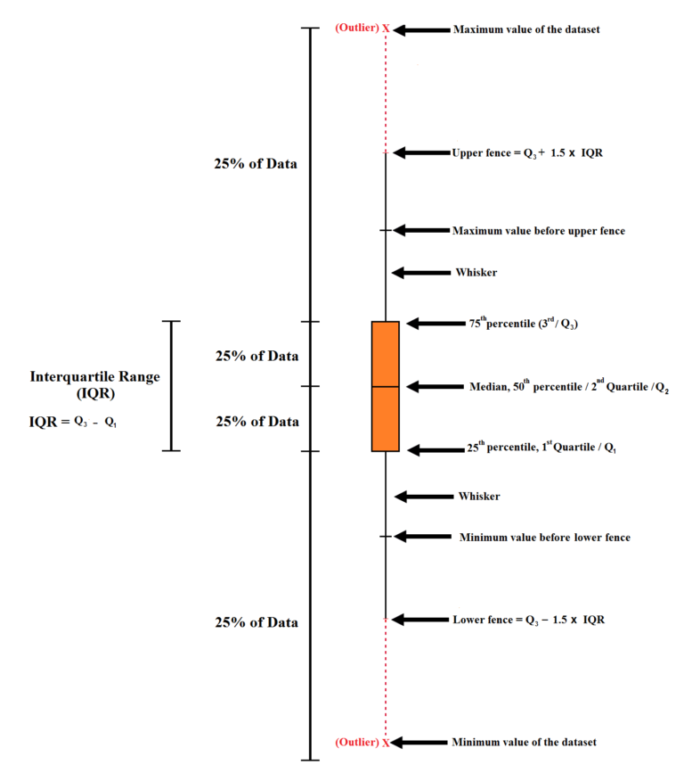
Here we are able to visualize the data points and see the outliers that lie far away. However, boxplots are not commonly used, as it takes a lot of time to cap outliers using boxplots if there are multiple features in a dataset. Also, other methods such as standard deviation and percentiles (discussed below) are equally reliable. Also, for creating boxplots generally a lot of data is required, and if there is an error while capping the outliers, we have to return to the boxplot all over again. Therefore boxplots are used in applications where high precision is required, such as chemical trials, risk modeling etc, where it takes weeks just to prepare the data. However, in other domains such as Marketing Analysis etc, other methods can be equally reliable.

Quartile Ranges

In a dataset, extreme data points are considered to be those 3 times the interquartile range below the first quartile or above the third quartile, whereas mild outliers lie between 1.5 times the interquartile range below the first quartile or above the third quartile.

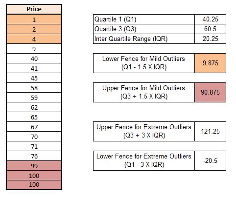
Here in the dataset, we have a few mild outliers. In this dataset, any value which is above 90.875 will be capped at 90.875, while any value below 9.875 will be capped at 9.875. In this dataset, we didn’t find any extreme outliers.

Quantiles / Percentile

Various percentiles can be used, ranging from P1 to P99, and for each variable, an arbitrary value can be taken where the percentile falls or jumps drastically. Before getting into that, it is important to be clear on the differences between quartiles, quantiles and percentiles.

0 quartile = 0 quantile = 0 percentile
1 quartile = 0.25 quantile = 25 percentile
2 quartile = 0.5 quantile = 50 percentile (median)
3 quartile = 0.75 quantile = 75 percentile
4 quartile = 1 quantile = 100 percentile

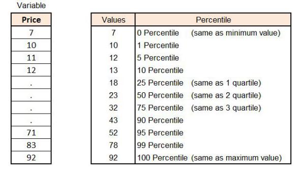
Here we can see how there is a sudden increase in the value at the 95th and 99th percentile, so we can use the value of the 95th percentile, which is 52, to cap the upper extreme values, while there is no major drop in the lower values, indicating an absence of extreme values (outliers) in the lower end.

Standard Deviation

Another common method of capping outliers is through standard deviation. Here generally data is capped at 2 or 3 standard deviations above and below the mean. For example, if we have a variable, then we can calculate the standard deviation of it, and by multiplying it by 2 and subtracting this value from the mean, we will get the value for the lower limit, while adding this value to the mean will provide us with the upper limit. The same can be done for 3 standard deviations, where we will multiply the standard deviation by 3 rather than 2.

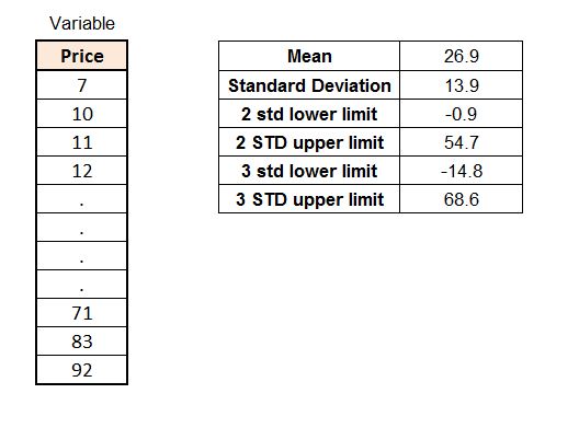
Notice how, when using the same dataset, the results come out to be similar to the percentile method, where we took 52 as the value to cap the upper value. Here also we didn’t find any lower extreme values. However, it can get difficult to decide between different values of STD, and for this, frequency tables can be used where the percentage of data will matter. For example, if we go with 2 STD then we find 5% of outliers, while with 3 STD we find 1% of outliers. When dealing with outliers, discretion is required. Here 5% outliers is an acceptable amount; however, if we would have found 10% of outliers with 2 STD, this could have meant that there are some natural extreme values, such as, in this case, the price of a commodity which is expensive. In such circumstances, we can take a different STD value, for example 2.5, and then see how much data is being considered an outlier. In practice, if we cap outliers using 3 STD, then using 2 or even 2.5 STD causing a large amount of data to become outliers indicates that the data is junk, meaning that the data is of very poor quality.

Methods such as clustering can be used, where the data points away from the clusters can be considered; however, it can take up a lot of time and is used when high precision is required. Transformation of data and binning the data also help in controlling the effects of outliers in the data. However, the above-mentioned methods are the most common methods for controlling the adverse effects of outliers.