// shared: regression & classification
Bagging
Bagging is a classic technique for generating a lot of predictors and combining them in a simple way. The word Bagging comes from Bootstrap Aggregating. Here we use the same learning algorithm but train each learner on a different set of data. Bagging is powerful as it can work with complex models such as a fully developed decision tree (it is in contrast with Boosting, which works with weak models).
Types of Bagging Methods
There are many ways of performing Bagging by tweaking the meta-estimators, such as:
Pasting
Here it creates bags (random subsets); however, in each bag, the observations (samples) are unique and are not repeated. This process is known as creating random subsets without replacement. The main drawback of this process is that each observation cannot be repeated in creating a bag, and this poses a challenge when the dataset is not large enough. Thus pasting is done only when the datasets are very large.
To understand this intuitively, suppose we have a dataset with 10 records. We first divide the dataset into train and test with 6 records (N) for training and 4 records for testing.
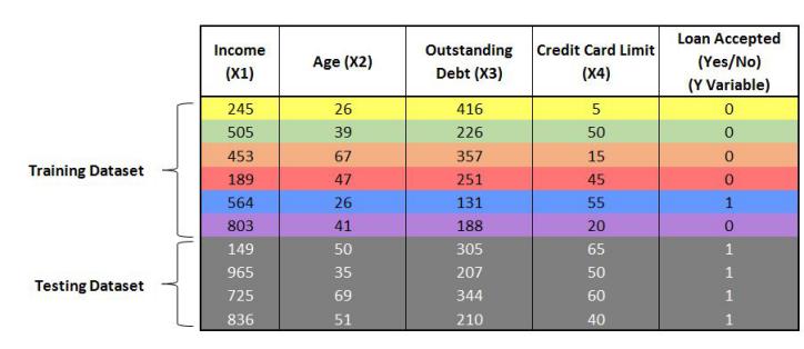
Now we have to create m number of bags (sub-sets) with each bag of size N’. The rule of thumb is that N’ should be less than N by 60%. Thus here we have to take 3 records to create each bag. The 3 records left each time while creating a bag are known as out of bag records. These out of bag records are used to validate the model in the training phase only (more on this under Random Forests).
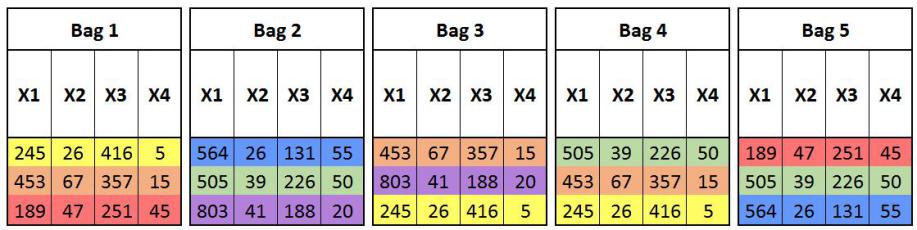
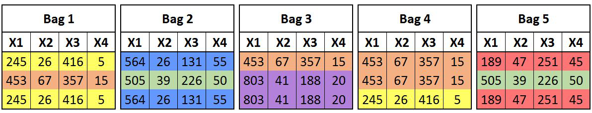
We now train a model on each of these datasets (for example, we use KNN as the learning algorithm) and consolidate this through majority voting to predict the Y variable.
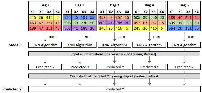
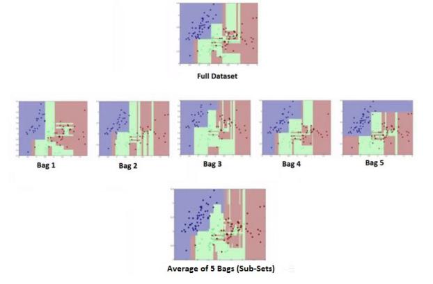
Thus we are able to calculate Y by subsets that all have unique records. The output will look something like this:
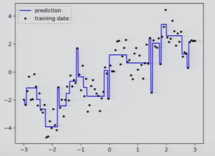
This output right now looks very complex; however, this can be reduced by increasing the number of bags.
Bootstrapping
It is the most common method and is simply called Bootstrap Aggregating, or Bagging. Here the sample is drawn with replacement, which creates a bootstrap sample, meaning that we create random subsets or bags with each bag having some duplicate records (observations/samples). This is a common statistical practice used to generate confidence values/confidence intervals of an estimate and understand what the variation does to the realisation of the dataset.
Random Subspaces
In this method of bagging, the subsets are created by randomly selecting features rather than randomly selecting observations as done earlier.
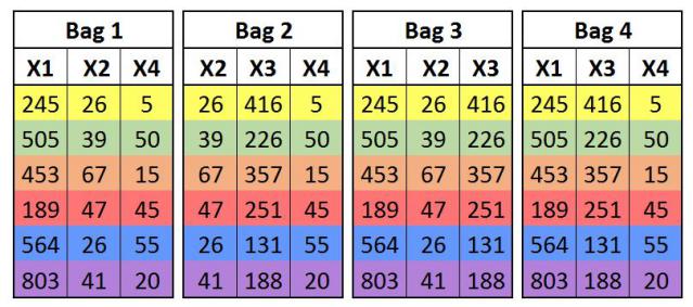
Here each bag is created by randomly selecting features rather than the observations (samples).
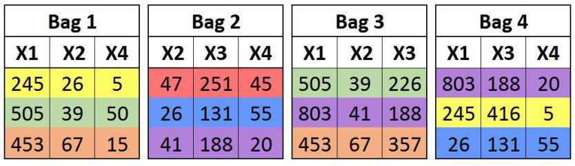
Random Patches
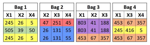
In this method of bagging, the subsets are created by randomly selecting both the features as well as the observations (samples). When running a statistical software, we are required to input the number of samples and the number of features to be used for creating bags (these inputs are known as hyperparameters and are found using grid search, etc.), along with whether we want to create subsets with or without replacement. We generally go for around 40-60% of samples and features when creating bags.
In this blog, we will mainly discuss bagging with bootstrap sampling (i.e. subsets drawn with replacement).
Reduction in Complexity by using Bagging
The whole purpose of using ensemble methods is to reduce overfitting, i.e. control the bias-variance by reducing overfitting of the data. As discussed in bias-variance, the model is overfitted when it memorises the training dataset. We have to control overfitting by reducing the complexity of the model. In bagging, the issue is addressed to some degree as, for example, if we are handling a classification problem, then it is harder for any bag of classifiers to memorise the data, since each one of the classifiers gets trained on its own individual training dataset, which was sampled from the original training dataset. As in each of these individual training datasets some data points (observations/samples/rows of a dataset) were deliberately left out, making it different from the original training dataset, this allows the model not to memorise the original training dataset, as the data point left out will be unavailable for the model to memorise. Therefore, even if the models created from these individual training datasets are highly overfitted, the ensemble will not memorise the left-out point, and when all these models are consolidated, it ends up providing us with an ensemble model that has an optimum complexity. Bagging uses averaging (for regression problems) or majority voting (for classification problems) for consolidating the different models.
Suppose we use fully grown decision trees as the learning algorithm to build models. Here each of these models will be extremely complex and overfitted. Suppose we begin with creating 5 bags and average them out to find the result.
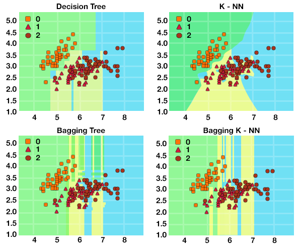 Decision Tree and K-NN compared against their bagged versions, Bagging Tree and Bagging K-NN, showing smoother boundaries after bagging">
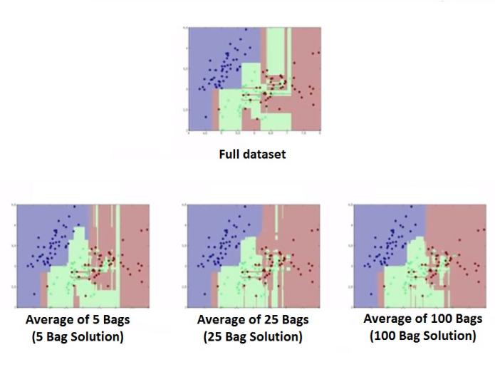
Here we see that after using bagging with a 5-bag solution, we are able to have less complexity when compared to the complexity of the original decision trees with all pure leaves. We can increase the number of bags for better results.
Here we can see that the complexity of the ensemble model decreases with an increase in the number of bags, even when each of the models is a fully grown, complex, overfitted decision tree. It also helps in increasing the accuracy of the model; for example, with classification, it lowers the misclassification rate of the classifiers.
Limitations of Bagging
It doesn’t work on predictors that are linear functions of the input data, since the average of a linear function will be another linear function. However, when there is a non-linear relation, or where we have a thresholded linear function, bagging can be used.
Other disadvantages include a lack of interpretability; unlike a simple decision tree, which can be read individually, ensemble methods work more like a black box and just produce the result.
Thus bagging is an effective way of addressing the issue of overfitting, and subsampling techniques do help in increasing the stability of the model. We can use different learning algorithms to create models, and can use bootstrap aggregating to come up with bags or subsets. The power of bagging can be extended for handling clustering problems, detecting outliers, etc. It can be used for variable selection by using decision trees, as in the final decision tree, the variables at the top 10 levels will be the 10 most important variables, since in the backend the bagging algorithm would have taken into account how many times a variable appeared in the top 10, and upon aggregating these findings we can get the important variables.
There are other alternatives to Bagging, such as Bragging, which stands for Bootstrap Robust Aggregating, often used with methods such as MARS (Multivariate Adaptive Regression Splines), as it yields better results than original MARS or Bagging MARS, and should also be explored.
Random Forests
Random Forest is a variation of the bagging algorithm which is designed specifically for decision trees, where it uses a combination of bootstrapping and random subspaces to form subsets of data. Random Forests can be of two types: Random Forest Regressor, used for Regression problems, and Random Forest Classifier, used for Classification Problems.
It is such a common application of bagging that it is considered a separate ensemble method; however, it is just a method of implementing bagging using decision trees. The other ensemble method for decision trees is known as Extra-Trees, which won’t be discussed in this blog.
Random Forest is better than using Bootstrapping with decision trees because, when applying Bagging to Decision Trees, the main drawback is that if we have a large dataset, then often the decision trees learnt from each of the bags (sub-sets) are not very different, often causing the separate decision trees to have the same root node. Thus, to diversify the models, we have to introduce some variability in the learner, which is done by selecting some features at every step of the decision tree training process (i.e. for every model, different features are selected).
Thus in Random Forests, we create subsets by selecting random samples with replacement, along with selecting random features without replacement. Thus each subset can have duplicate samples (observations); however, there are randomly selected features which are unique. Separate, highly complex decision trees are built on these subsets and are consolidated to give us a less complex, less overfitted ensemble decision tree which also has optimum accuracy.
One must note that we can create as many trees as we want in an ensemble model; however, after a point, there are diminishing returns, and it will take unnecessary time to compute the result. The important parameter here is the number of features, which can be taken as the square root of the number of features, or 40-60% of the number of features. Also, if the dataset is very large, then it may not be a good idea to have a fully grown tree for creating different models, so we can tune the parameters to limit the growth of the trees, as doing otherwise will take a lot of time and consume a lot of computational memory.
Random Forests are effective when the dataset is in very high dimensions, has outliers or missing values, or if the classes are unbalanced. Their effectiveness outperforms Adaptive Boosting (discussed in the Boosting article) when dealing with outliers.
Out of Bag Error
One of the biggest advantages of Random Forests is that it can eliminate the traditional method of validating a model, which is done by keeping aside a portion of data for testing, training the model on a training dataset, and then applying the model to the testing dataset to see its accuracy. This is done by using Out of Bag Error, or OOB Error (also known as out-of-bag estimate), which is a method of measuring the prediction error for Random Forests, boosted decision trees, and ensemble models that utilise bootstrap aggregating to form subsets of data for training. OOB error computes the error for each model from the data points that were not included in the bootstrap sample. Sub-sampling allows defining an out-of-bag estimate of the prediction by evaluating the prediction on those observations which were not used in building the model. A study by Leo Breiman (creator of the bagging method) has shown that the out-of-bag estimate is as accurate as using a test set of the same size as the training set, thus avoiding the need for an independent validation dataset and allowing us to use the whole of the data for creating Random Forests. In various software, we can set oob_score=True (in Python), where the model computes the out-of-bag error while building the Random Forest.
Bagging, which mostly refers to Bootstrapping using Decision Trees, is a great ensemble method and is commonly used. Random Forest, which is a great application of the Bagging method, can be used for large, complex datasets; however, it tends to be more effective for classification than for regression (in a regression problem it cannot predict beyond the range of values seen in the training data), and also, as discussed earlier, it works like a black box, giving little control over the process apart from the control provided by the hyperparameters. Compared to Boosting methods, Bagging doesn’t have the advantage that different Boosting methods have, which is working particularly on those observations where the error is high. Nonetheless, it is among the most commonly used ensemble methods.