// shared: regression & classification

Boosting

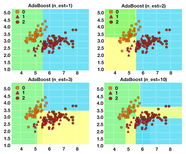
Boosting is another ensemble method that often gives better accuracy than bagging, but it might give an overfitting problem if we don’t know where to stop the process. There are three types of boosting: Ada Boost (Adaptive Boosting), Gradient Boosting, and XGBoost (Extreme Gradient Boosting).

Ada Boost (Adaptive Boosting)

Bagging is a parallel process, while adaptive boosting is sequential, where the next model is based on the current model.

Thus the major difference between bagging and boosting is that with bagging we created m number of bags, each having randomly selected observations, while in boosting, the observations of the bag are affected by the performance of the model on the previous bag. Here, unlike Bagging, we use weak learners (i.e. models such as very shallow decision trees). The predictions of these weak learners are combined using a weighted average (for regression problems) and weighted majority voting (for classification problems), unlike bagging, where a simple democratic method was used, as here the models that show good performance during training are rewarded by giving them higher weights than the model which had a higher error rate.

Process

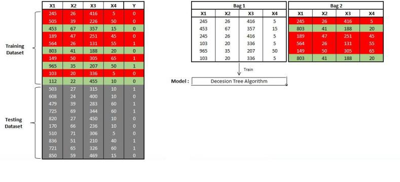
Suppose we have 20 observations of a classification problem, out of which we take 10 as the training dataset for creating the Ada Boost Model. Out of these 10 observations, the first bag is created by randomly selecting 6 observations (drawn with replacement), and the dataset is used to learn a decision tree algorithm. However, unlike bagging, all the x variables and the 10 observations of the training dataset are used, and the model is applied. We find that out of the 10 observations, the Y variable for 6 observations was predicted wrong. We create another bag; however, this time we add weights to the observations that we wrongly classified, and we pay more attention to these observations, and the chances of these observations being considered for creating the next bag increases. This process takes place until the number of bags specified is created.

Here in a two-bag solution, of the 6 records that are incorrectly classified, 4 of them make it to the next bag. Thus initially the weights are the same for all the observations (1/N); however, as the model proceeds, the weights of the incorrectly predicted observations are increased, whereas the weights for the correctly predicted observations are decreased, and each weak learner is forced to pay attention to those observations that were either missed by the previous model or were not predicted correctly.

Gradient Boost

In this process, we scale up the complexity with each iteration. Here in each stage, the error in each model is computed, which is the gradient of the loss function. In the next stage, the new model compensates for the shortcoming of the previous weak model. These shortcomings are the errors, or gradients (of the loss function). Notice here, unlike adaptive boosting, the errors are not identified by providing them weights and using them to create new buckets; rather, here the training data is used (here training and testing/model evaluation is done not by bootstrapping, as done in bagging/random forest, where all the data can be used and out-of-bag error can then be used to evaluate the model, but is done through k-fold cross-validation, where each fold is regarded as the test set and their average is used to measure the final performance) to identify the data points that were difficult to predict (i.e. had large residuals) by the initial weak model, and are made to correct the error by making the model more complex. Gradient boosting can be used for Regression as well as Classification problems; however, from an understanding point of view, Regression using Gradient Boosting can be easily understood.

For example, we have a regression problem, and on a dataset we perform gradient boosted trees.

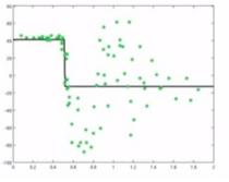
We fit a one-layer decision tree and get an output something like this:

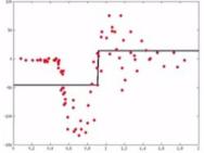
However, it is a very simple model, and we can see there are a lot of errors (particularly on the top-left side of the graph). Thus the gradient boosting algorithm computes the gradients of the loss function.

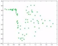
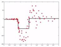
On the basis of the error residual function shown above, a new simple model is created (here it is being created by fitting a single-layered decision tree) to predict the error residuals.

Here we end up predicting new data points with improvement. We successfully predict those data points that were predicted incorrectly by the previous model (top-left side of the graph).

We can add these two predictors and come up with a new model, which is more complex than the single model we were using, but has a lower overall error.

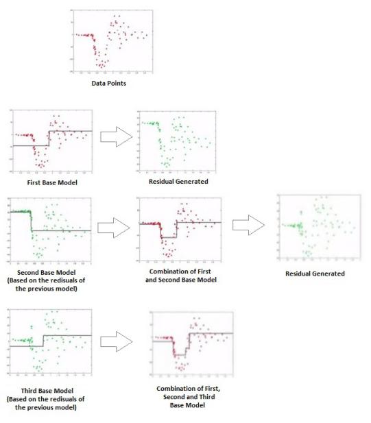
Thus we use a number of weak learners and boost them into a strong learner, where each weak learner trains on the errors left by the previous weak model, and by using a gradient descent optimization process, we combine these weak models to come up with a relatively strong, complex model.

We can continue this process by computing the error residuals of the more complex model and can create another weak model where it will try to minimize the large error residuals, and by combining that weak model with the earlier two weak models, we can come up with a stronger, even more complex model which will have lower residuals than the previous model.

One of the disadvantages of Gradient Boosting is scalability, as due to the sequential nature of boosting, it cannot be parallelized.

Extreme Gradient Boost

Extreme Gradient Boosting (XGBoost) is a more advanced form of gradient boosting. It performs 3 types of gradient boosting: Standard Gradient Boosting (discussed above), Stochastic Gradient Boosting (sub-sampling is done at the row and column level), and Regularization Gradient Boosting (L1 and L2 Regularization are performed). It is a scalable machine learning system and is so powerful that out of the 29 machine learning challenges organised by Kaggle (a machine learning competition site), winners of 17 challenges used XGBoost; of these, 8 used XGBoost on its own, while most of the others combined XGBoost with neural networks in their ensembles. The advantage of XGBoost over standard Gradient Boosting is that it is a parallel learning technique and saves time when compared to standard Gradient Boosting (it is parallelized by using all of the CPU cores during the training process). It also helps in handling overfitting, as it uses both regularization techniques (L1 and L2 regularization), and is more effective with missing values (sparse awareness). Cross-validation is done at each iteration, generally by using k-fold validation (e.g. k=10), where each of the ten folds is regarded as the test set and their average is used to measure the final performance. It is important to note that XGBoost uses a lot of hyperparameters which are to be optimised, especially the number of base models that are to be created, as after a point it will end up creating a fairly complex, overfitted model.

Generally, XGBoost is used as a Scalable Parallel Tree Boosting Ensemble method and is among the most famous methods for performing classification and regression.

Boosting is another great ensemble method where the output of the previous model affects the next model. Thus here the function is learned sequentially. The basic difference between bagging and boosting is that bagging is a parallel ensemble, where each model is built independently, while boosting is a sequential ensemble, where we add new models to do well where the previous models lack (however, boosting can be done in parallel by using Extreme Gradient Boosting). Also, both address the bias-variance problem, with bagging having the aim of decreasing variance (very complex base models are used, and thus bagging is suitable for reducing the complexity/overfitting of complex models), while the aim of boosting is to decrease bias (very simple base models are used, and thus boosting is used to systematically increase the complexity of the model).