// inferential statistics

Correlation Coefficients

Correlation coefficients are one of the most commonly used statistical tools which is used when we want to know if the two variables in question are related to each other or not. It also allows us to know about the magnitude of this relation. There are many types of correlation coefficients but one of the most common is the Pearson product-moment correlation (Pearson’s correlation / Pearson’s R) and is heavily used in Linear Regression. To use this correlation method, both the variables must be numerical (continuous) variables.

Direction of Correlation Coefficients

The most basic and fundamental characteristic of coefficients is its direction. There can be two directions for a correlation coefficient- positive or negative.

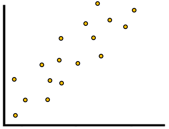
Positive Correlation

It means that two variables move in the same direction, so for every unit increase in variable 1, there is an increase in variable 2.

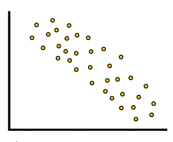
Negative Correlation

It means the two variables move in the opposite direction, so for every unit increase in variable 1, there is a decrease in variable 2.

Magnitude of Correlation Coefficients

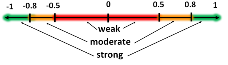
The strength of the Correlation can be determined which ranges from -1.00 to +1.00. In Pearson coefficient, ‘r’ is the symbol for the coefficient and its value determines the magnitude of the direction of the correlation.

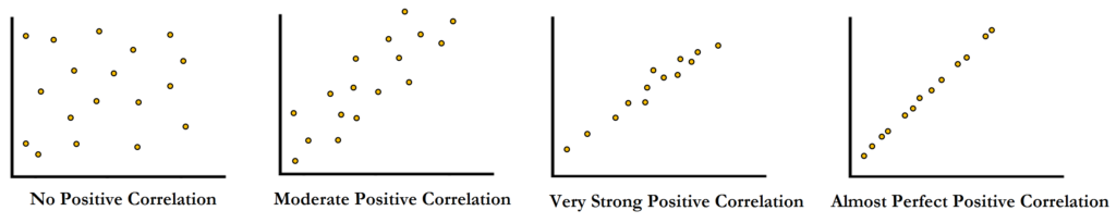
1 to 0

1 indicates a very strong positive relationship. That means for every unit increase in Variable 1 there is a proportional amount of increase in Variable 2. The positive correlation can vary from 0 to 1.

r = 1 - Perfect Positive Correlation
r = 0.8 - Very Strong Positive Correlation
r = 0.5 - Moderate Positive Correlation
r = 0.3 - Weak Positive Correlation
r = 0 - No Positive Correlation

If the r > 0.5 then it is considered to be correlated, however this decision can be very subjective.

-1 to 0

-1 indicates a very strong negative relationship. That means for every unit increase in Variable 1 there is a proportional amount of decrease in Variable 2. The negative correlation can vary from 0 to -1.

r = -1 - Perfect Negative Correlation
r = -0.8 - Very Strong Negative Correlation
r = -0.5 - Moderate Negative Correlation
r = -0.3 - Weak Negative Correlation
r = 0 - No Negative Correlation

0 (Zero)

0 means that there is no relation between two variables and for every unit increase in variable 1 there can sometimes be an undefined increase or decrease in variable 2, showing no signs of correlation.

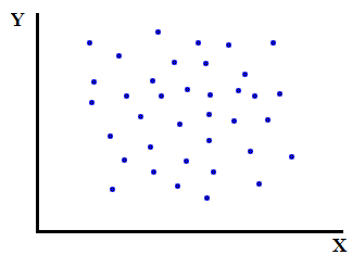
Example of no correlation can be the average speed of your car and the number of wildfires that happen in the world. There is (probably) no relation between them.

Calculating Correlation Coefficients

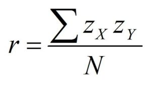
There are several different ways to calculate correlation coefficients. To calculate Pearson’s Correlation Coefficient, the data has to be standardised. The sum of the cross product between the z scores of the two variables is calculated, i.e. multiply each standardised score on one variable with the standardised score on the other, sum all of this and divide it by the number of pairs (N). Because the scores are standardised (z scores), this directly gives the correlation coefficient. (Using the raw mean-deviations instead would give the covariance, which becomes the correlation coefficient once standardised.) In the below-mentioned formula, we simply standardise the variable first before we find a cross product.

Negative and Positive correlation coefficient is produced when for example an individual case has a score below the mean in variable 1 and 2, their cross product will produce a positive value (when two negative values are multiplied the outcome will be positive), similarly if the score was positive in both the variables (above the mean) they also produce a positive value. This is how we get a positive coefficient. If the individual case has a positive value in variable 1 (the value is above the mean of variable 1) and a negative value in variable 2 (the value is below the mean of variable 2) then their cross product produces a negative value (positive value multiplied by negative value produces a negative output) and this is how we get a negative coefficient.

Determining Statistical Significance of Correlation Coefficients

To determine if the given value of Correlation Coefficient is statistically significant or not, T distribution can be used. The formula for finding the t value is t = r-p ÷ sr where r is the sample correlation coefficient, p is the population correlation coefficient and sr is the standard error of the sample correlation coefficient. So that we don’t have to separately calculate the standard error and then use it as the denominator, a simple formula can be used-

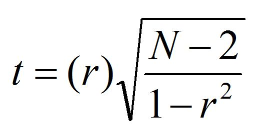
Here the degree of freedom is N-2 and with the t value and degree of freedom, the statistical significance can be found by using the t table.

Coefficient of determination (R² / R-Square)

To determine if the given value of correlation coefficient means a strong relationship between variables, coefficient of determination can be used. Coefficient of Determination, also popularly known as R-Square (symbol- ‘R²’), will be used commonly especially in Linear Regression to assess how well a model explains and predicts future outcomes.

Coefficient of Determination breaks down the question to- if the variance found in variable 1 is associated with variance found in variable 2. Thus coefficient of determination is used to explain how much variability of one variable can be caused by its relationship to another variable, i.e. how much of our correlation coefficient is able to explain the variance found in one variable based on the score found in the other variable. Coefficient of determination can be understood in a way that when two variables are correlated, they also share some amount of variance and a stronger correlation means a higher percentage of variance shared among them. The precise amount of shared (explained) variance is calculated by squaring the correlation coefficient (r) that provides us with Coefficient of Determination (r²).

Limitations of Correlation Coefficients

The problem of truncated range can happen such as when one or both the variables in question don’t have much variety in the distribution (due to ceiling or floor effect). For example when trying to find a relationship between the number of hours a student studies and the marks obtained by the student. There can be a scenario where there is variation in variable 1- time spent in studying but there is not much variation in variable 2- marks obtained by students as everyone scores high marks (causing a ceiling effect).

Also, correlation coefficient is not able to tell from the two variables used, which one is the dependent and which is the independent variable. So two variables can be correlated, for example having a Correlation Coefficient of 0.6, however, the same result will be found if the two variables are switched. If a 0.6 correlation is found between junk food and obesity then one can say that the higher the amount of consumed junk food, the higher are the chances of obesity, however if the variables are switched, the correlation will be the same but the result will be ‘obesity causes junk food’ which makes no sense and thus independent and dependent variables are to be kept in mind. The word ‘cause’ used earlier is also of much importance and should be used keeping a lot of factors in mind as correlation doesn’t explain causation. Correlation simply means whether, on average, the values on one variable are associated with the other variable or not, however causation means that the increase/decrease (variance) in scores of one variable is because of (caused by / created by) the variance in another variable. Example- one can say there is a positive correlation between longer days and happiness, however, it is just a correlation and not necessarily that longer days make people feel happy, and other factors can be involved such as longer days being in summer, and if the sample was collected from a non-tropical country then the happiness is caused by summer and not by longer days itself. Thus correlation does not provide enough evidence to draw a causal relationship between two variables and conclude that there is a cause and effect relationship between them.

Pearson’s Correlation Coefficients are meant to examine the linear relationship among variables, however, if the relationship is curvilinear then the correlation coefficient produced from such a relationship is very small, indicating no or very little relationship among variables when a strong relationship may actually exist.

Example of a Curvilinear relationship can be of anxiety and exam score, where with the increase in anxiety there is an increase in the score obtained by students, however when anxiety goes beyond a certain point then the score starts to fall (negative correlation). Thus in a Curvilinear Relationship, one variable increases and so does the other variable, but only up to a certain point after which when one variable increases, the other decreases.

Other Type of Correlation

There are other types of correlation coefficients also, such as Point Biserial, where unlike Pearson’s coefficient, one variable is continuous and the other is two-level categorical. Example- if studying maths in college (Y/N) has a relationship with marks in a standardised aptitude test. Spearman’s Rho is a non-parametric test used to measure the strength of association between two variables and is used when data is recorded in ranks, and as ranks are a form of ordinal data, Pearson Correlation Coefficient cannot be used. Example- if rank attained in college is related to marks in a standardised aptitude test.

Pearson’s Correlation Coefficient is very helpful in explaining relationships shared between two variables. However, there are other inferential statistics that can be used such as t-Tests and F-tests when we require to find the relationship between variables where all variables are not necessarily numerical or may have multiple variables etc.