// time series

Averaging Techniques

Time series models are created when we have to predict values over a period of time, i.e. forecasting values. There are multiple techniques to do this. In this blog, the most basic techniques, known as Average Models, are explored. Such models are used when we don't have any major pattern in our data and the number of data points is not large enough.

There are multiple types of Average Models: Simple Average Models, Moving Average Models and Weighted Average Models. We will use a univariate dataset to explore all of the above-mentioned models and understand how they work.

Simple Average Technique

To understand Simple Average Technique, we consider a dataset with one variable, Price, which is indexed by time where the time interval is in quarters.

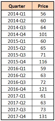
Now, if we want to predict the price for 2018-Q1 using Simple Average Technique, we simply take the average of the price, which comes out to be 77.25 (1236/16).

If we plot the data points on a graph, we can see a pattern where there is a slump in the price at every first quarter while the price peaks at every fourth quarter, while the overall trend is positive.

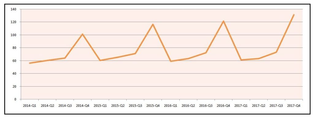
Thus here two concepts are present - Seasonality and Trend. We cannot be sure of the third, Cyclicity, as to determine that we need to have more data points (for example, data from the last 7-8 years).

We have used a simple moving average, which makes the graph look something like this:

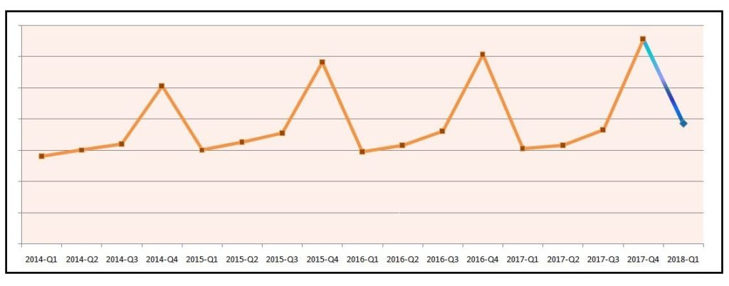
However, as there are trend and seasonality in our data, we require a method which can capture this in a better manner, which brings us to the next technique.

Moving Average Models

In Moving Average, rather than taking the average of the whole variable, the average moves over time. For example, for Q1 it can be 12, while for Q2 it can be 14.

If we take the above example and have to predict the value for 2018-Q1, then we first need to know the specific number of periods over which the average is to be taken. For example, if we decide to consider the average of the last four quarters, then the forecast for 2018-Q1 will be 82, which is different from the 77.25 we got when we used the Simple Average Technique.

However, there is one major drawback with this method, which is giving the same importance or weight to all the values of the past period. However, by taking a quick look at the dataset, it can be understood that the recent values should have higher weightage, and also that higher weightage should be provided for specific time periods. To resolve this issue, we use a technique called Weighted Moving Average.

Weighted Moving Average

In situations where we know that certain time periods have higher weightage, we use Weighted Moving Average, where we give weights to specific data points.

For example, taking an average of the last 4 quarters: if we use the above dataset, then for forecasting the value of 2018-Q1 we take the average of 2017-Q1, Q2, Q3 and Q4. However, instead of simply taking a moving average, we assign weights to them. If we decide to give a weight of 0.4 to 2017-Q4, 0.3 to 2017-Q3, 0.2 to 2017-Q2 and 0.1 to 2017-Q1, then the result comes out to be 93 ((61×0.1)+(63×0.2)+(73×0.3)+(131×0.4)).

It is important to note that in this example the sum of our weights was 1. If we use weights such as 4, 3, 2, 1, then we multiply the prices by these weights and divide by the total of the weights, i.e.

= ((61×1)+(63×2)+(73×3)+(131×4))÷(1+2+3+4)
= (61 + 126 + 219 + 524) ÷ 10
= 930 ÷ 10
= 93

Deciding Period

There also comes the question of deciding the number of periods to be considered for calculating the moving averages. So far in this blog we have taken only the last four quarters to calculate the average; however, it is possible to get a better forecast by using the last three quarters or five quarters. To get an idea of which time period is better, we forecast the already-available data using different time periods and calculate the error using various error measures; the time period selected for forecasting is the one that provides the minimum error.

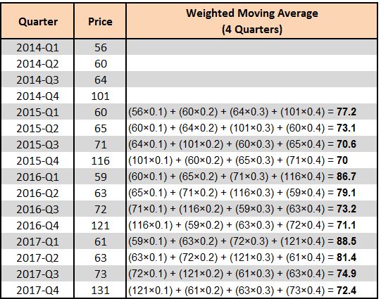
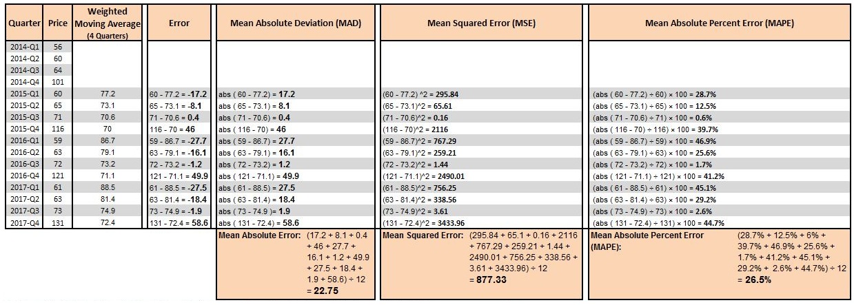
To understand this, we first apply weighted moving average on our data by considering the last four quarters and taking weights 0.4, 0.3, 0.2 and 0.1.

Methods of Calculating Error

We forecast using the above-mentioned weights and consider the last four quarters to get the results. Now we calculate the error. We can use various error measures to do so, such as Simple Error, Mean Absolute Deviation, Mean Squared Error and Mean Absolute Percent Error.

Simple Error: Actual − Forecast.

Mean Absolute Deviation (MAD): Here we use the absolute value of the simple error and then take an average of all these errors.

Mean Squared Error (MSE): Here we square all the errors and then take the average of them.

Mean Absolute Percent Error (MAPE): It is calculated by dividing the absolute value of the simple error by the actual value, then multiplying it by 100 to get the result in percentage.

Above we calculate various error measures using the forecasted values calculated by considering the last four quarters. If we do the same process, but this time forecast by considering only the last five quarters (using 5 weights: 0.35, 0.25, 0.2, 0.15, 0.05), then we get the following results:

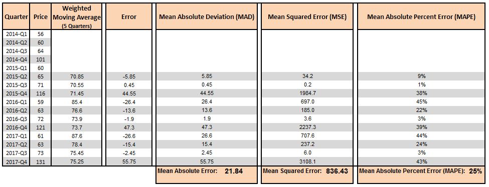
We can see that by considering the last five quarters we get better results, as the various error measures are lower. Thus, by considering the last five quarters and forecasting using weights 0.35, 0.25, 0.2, 0.15 and 0.05, the forecasted value for 2018-Q1 comes out to be 91.9.

Deciding Weights

Deciding the weights can be done by using various optimization techniques, i.e. using a different combination of weights, checking the errors, and selecting the combination that provides the best result (minimum error). As only a limited number of manual iterations are possible, we can use linear programming techniques. In Excel, a simple function called 'Excel Solver' can help us in finding the correct combination of weights.

Average Models are very helpful, as they are easy to understand and implement; however, they are not as robust as techniques such as Smoothing Techniques and Time Series Decomposition, mentioned in the next blog.