// clustering problems

DBScan

DBScan is a density-based clustering method, also known as Density-Based Spatial Clustering of Applications with Noise. As the name suggests, it can handle outliers and noise in the data and can create clusters of arbitrary shapes. In DBScan, clusters are formed by connecting the data points that are densely located in a region.

Epsilon and MinPts

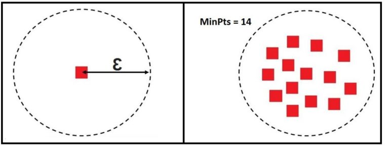
The two most important parameters for DBScan are ε (Epsilon) and MinPts (Minimum Points). ε is the radius of the neighbourhood of a data point, while MinPts is the minimum number of data points that should be there in a neighbourhood in order to consider the neighbourhood dense enough to be a cluster. In very simple terms, ε decides the size of a circle, and MinPts decides the minimum number of data points required to be in that circle to consider it a cluster.

Two circles illustrating Epsilon as the radius of a neighbourhood and MinPts as the minimum number of data points, 14, required within that neighbourhood

Core Point, Border Point and Noise Point

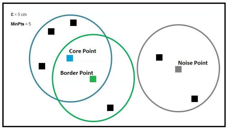
When using DBScan, the data points are categorised into three types: Core Point, Border Point and Noise Point. A data point is called a core point when it has the predetermined MinPts in its ε neighbourhood. A data point is categorised as a border point when it doesn’t have the minimum required data points but has one or more core points in its ε neighbourhood. A data point is a noise point when it has neither the required minimum number of points nor a core point in its ε neighbourhood, and such a data point is regarded as an outlier in the data.

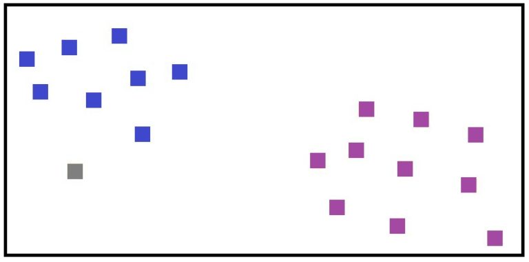
Below we can see that for ε=5cm, MinPts=5, the blue square is the core point, the green square is the border point and the grey square is the noise point.

Diagram with epsilon equal to 5 centimetres and MinPts equal to 5, showing a blue core point, a green border point, and a grey noise point inside their respective neighbourhood circles

Creating Clusters using DBScan

By using the above-mentioned concepts, DBScan is able to create clusters where, using interconnected neighbourhoods, it is able to assign a cluster to the data points that are densely located in a region. Here clusters are formed by choosing a random uncategorised point, and once it is found to be a core point, the algorithm labels the core point and the points in its neighbourhood as part of a cluster.

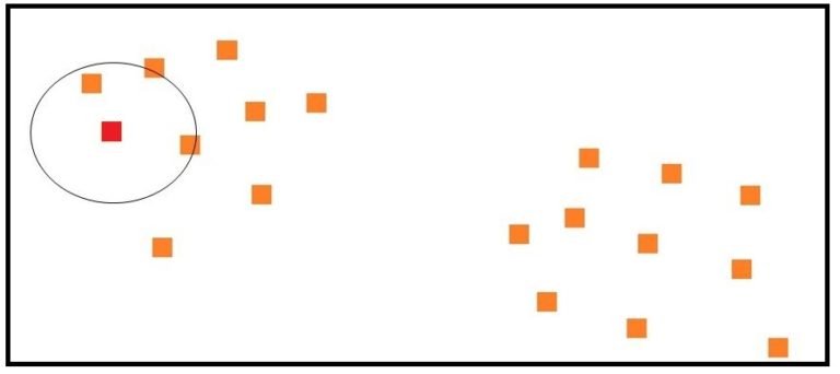
Scatter plot with a randomly selected point circled, identified as a core point because of the data points within its neighbourhood

In the above figure, MinPts is set as 3, so the randomly selected point is considered to be a core point as it has 3 data points in its ε neighbourhood. This data point and the data points in its neighbourhood are provided with a cluster label ‘A’ (blue square). Now, to find all density-reachable points, the algorithm jumps neighbourhoods and assigns them the same cluster label, i.e. for the data points that are beyond the neighbourhood of this core point, we find if these data points are core or not. If they are found to be core data points, then the data points in their neighbourhood are also labelled with the same cluster label.

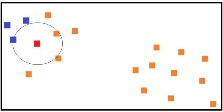
Scatter plot with the original core point's neighbourhood expanded, several additional points now labelled blue as part of cluster A

This is done with all the data points, and a cluster is found when strings of directly density-reachable data points are found, where a data point is directly density-reachable to B, B is directly density-reachable to C, and so forth.

We can see in the image below the neighbourhood for all the data points, with the core points being in red, border points in green, and outliers in grey.

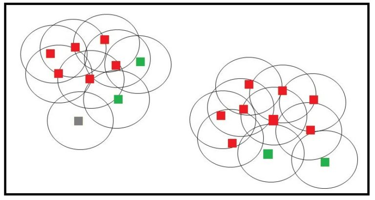
Scatter plot with overlapping neighbourhood circles around every point, showing chains of directly density-reachable points forming two groups

Thus we are able to come up with two clusters, while the outliers are left out of any clusters.

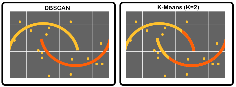
Two clusters of overlapping neighbourhood circles, each with red core points and green border points, and one grey noise point left out of both

DBScan is effective when we have outliers in the data, as unlike K-Means, it doesn’t get affected by outliers since it has no centroid that needs to be updated. DBScan is helpful in finding clusters of various sizes and shapes. A typical example of this is when the data is in the shape of a half moon, where K-Means, because of noise, gets adversely affected, whereas DBScan remains unaffected.

Side-by-side comparison of DBSCAN and K-Means with K equal to 2 on a half-moon-shaped dataset, with DBSCAN correctly separating the two crescents and K-Means splitting them incorrectly

However, it is important to take care of the parameters, as if we have a very low ε, then fewer points will be directly density-reachable, and a lot fewer clusters will be formed, as sparse clusters will be labelled as outliers, while a large value of ε will cause a lot of points to become directly density-reachable, which may cause outliers to be included in the clusters and dense clusters of data points to merge. Also, DBScan is not very effective when the data is in very high dimensions. However, it can be faster than some other clustering algorithms and should be used when the dataset has noise.