// clustering problems

Hierarchical Clustering

Hierarchical clustering is a Hard clustering method where, unlike K-Means (which is a Flat clustering method), we don’t pick a set number of clusters but rather we arrange the data in a hierarchy, where on top of the hierarchy we have a single big cluster while at the bottom of the hierarchy we have as many clusters as observations the dataset has.

Agglomerative v/s Divisive Clustering

There are multiple ways of building a hierarchy, but the two most famous methods of hierarchical clustering algorithms are Agglomerative Hierarchical Clustering Algorithms (AGNES) and the Divisive Hierarchical Clustering Algorithm (DIANA).

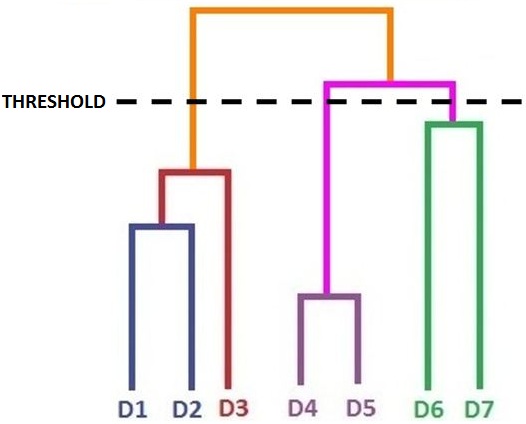
Below is a dendrogram, which is a common way of representing a diagram of hierarchical trees of clusters. By looking at it, the difference between agglomerative and divisive clustering can be easily understood.

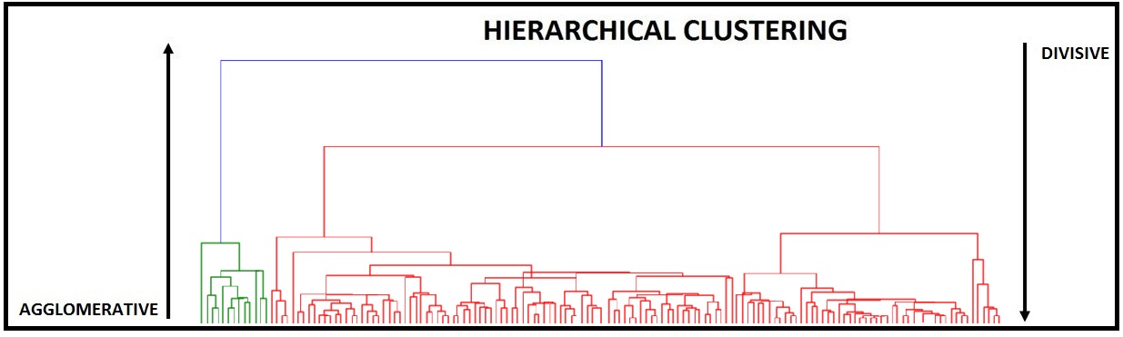
Agglomerative Hierarchical Clustering Algorithms (AGNES): It is a bottom-up approach where we initially assign different clusters to each observation, and then, on the basis of similarity, we consolidate/merge clusters until we are left with one single cluster.

Divisive Hierarchical Clustering Algorithm, aka Divisive Analysis Clustering (DIANA): The opposite of the agglomerative method is the divisive method, which is a top-down method where initially we consider all the observations as a single cluster. We then divide this one big single cluster into smaller clusters. The clusters can be divided continuously until we have one cluster for each observation.

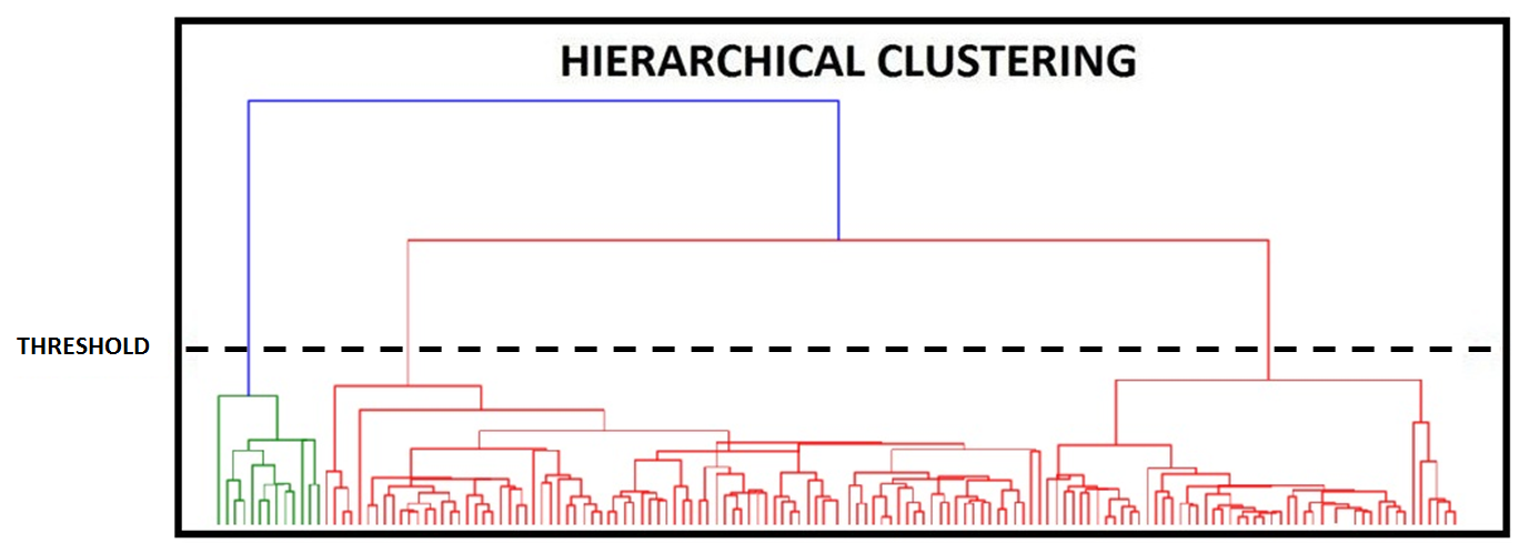
In both methods we use a threshold which provides us with a number of clusters. If our threshold is high, we get closer, more generalised clusters, while if our threshold is too low we can get a lot of clusters which are too fine-grained to be of any meaning. This threshold can be visualised as a cutoff point on our dendrogram, where the basis of the threshold can be dissimilarity.

Types of Linkages

As mentioned above, in both methods we either require finding the similarity (agglomerative method) or dissimilarity (divisive method) among the clusters. This is done by calculating the distance between the clusters. There are multiple ways of calculating this distance, such as Single Linkage, Complete Linkage and Average Linkage.

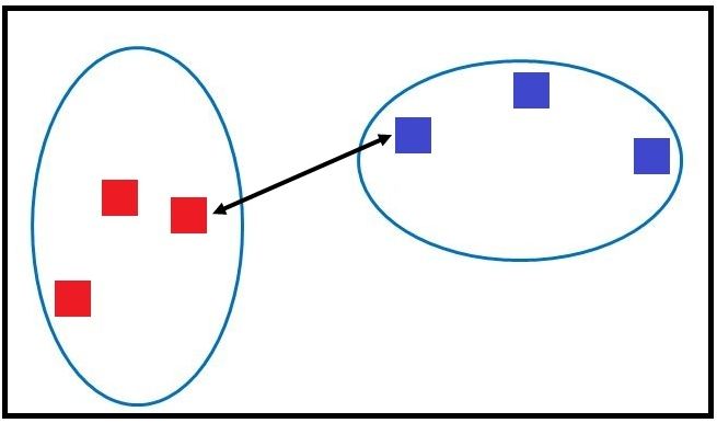
Single Linkage (Nearest Neighbour)

When we perform clustering using single linkage, we find the proximity between the two clusters by calculating the shortest distance between them. Here we consider the two closest data points of the two clusters to calculate the distance.

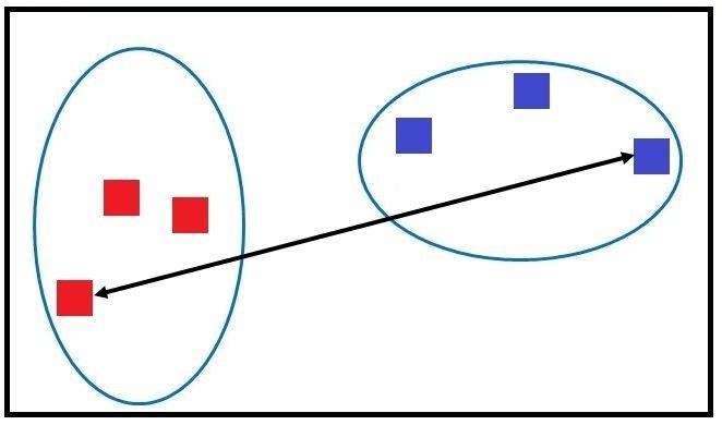
Complete Linkage (Furthest Neighbour)

It is the opposite of Single Linkage, where we consider the two farthest points of both the two clusters. Thus we take the maximum distance between the two clusters to find the proximity between them.

Average Linkage

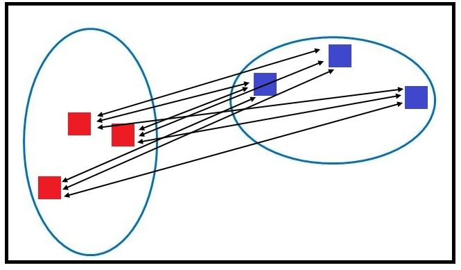
Also known as the Unweighted Pair Group Mean method, here, unlike Single and Complete Linkage, we consider the average distance. For this, we calculate the average distance from each data point of a cluster to all the data points of the other cluster.

There are other methods, such as the Centroid Method, where the centre points of the clusters are used to measure the distance between them. Another famous method is Ward’s Method, where the sum of squared Euclidean distance is minimized (minimum variance), i.e. the error sum of squares over all the observations of the two clusters is used to find the proximity between the two clusters.

So far we have discussed two types of clustering: Agglomerative and Divisive. As both methods are mirror opposites of each other, only one will be discussed in detail here. In this article, agglomerative clustering will be explored using the Single, Complete and Average Linkage methods.

Agglomerative Hierarchical Clustering

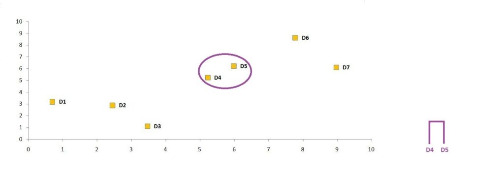
To understand in detail how agglomerative clustering works, we can take a dataset and perform agglomerative hierarchical clustering on it using the single linkage method to calculate the distance between the clusters. For example, we have a dataset with two features, X and Y.

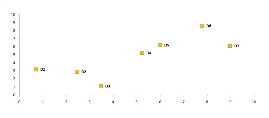
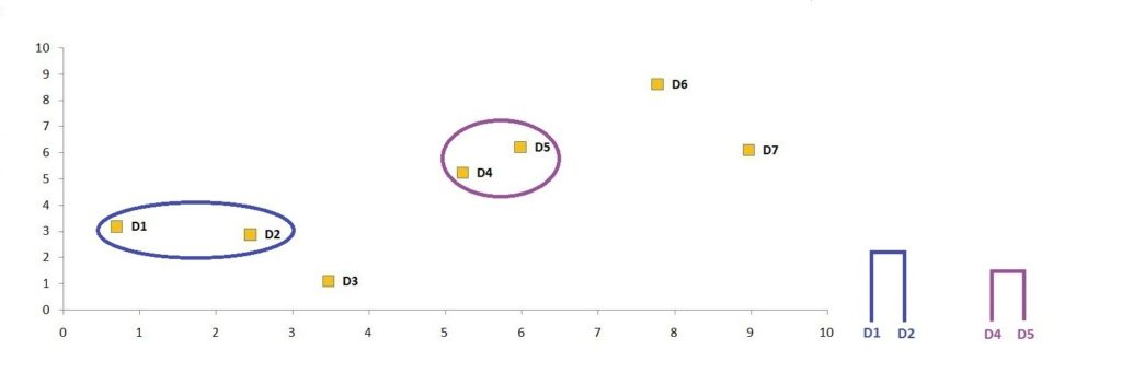
When the data points are plotted on the x and y coordinates, we get the following graph:

To perform hierarchical agglomerative clustering, we will perform a number of steps where we start with as many clusters as observations we have in the dataset, which in our case is 7. Therefore, right now we have 7 clusters. Now our goal is to perpetually consolidate the data points to form clusters until we are left with a single cluster.

Steps for Performing Agglomerative Hierarchical Clustering

Step 1: We first create what is known as a distance matrix. Here we compute the distance from each observation to all the observations of the dataset. The distance metric that we are using in this example is Euclidean distance.

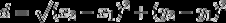
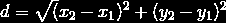
The formula for Euclidean distance is:

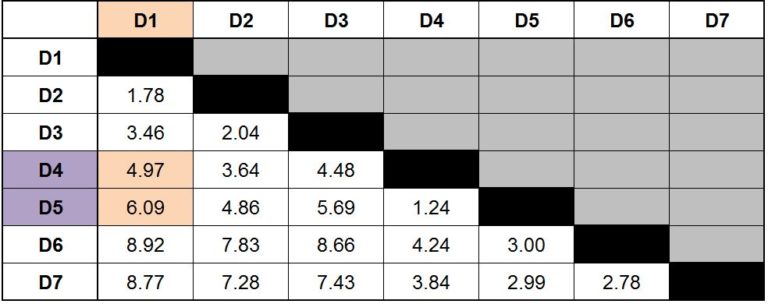
By using the above formula we calculate the Euclidean distance from each observation to all the other observations and come up with the following table.

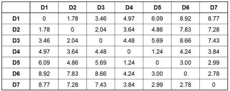
If we look closely, the distances in the upper and lower fold of the distance matrix are the same. Also, if we look diagonally, we notice that there are 0s - for example, when we calculate the distance from D1 to D1, we have 0 distance, similarly from D2 to D2, and so forth, thus the distance is nil.

Therefore, for the sake of simplicity, we remove the duplicates and 0 values and come up with a simplified distance table.

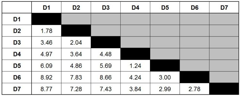
Step 2: As mentioned at the beginning of this article, agglomerative clustering is a bottom-up approach; therefore, we merge observations together based on their similarity (minimum distance). We look at the table to find those data points that are closest to each other.

We look for the minimum value in our table and find that the minimum value is 1.24, which is the distance between D4 and D5. Therefore, the two closest data points in the dataset are D4 and D5. Thus we merge these two data points to form a cluster. We can now visualise this cluster on the graph and create a dendrogram for it.

Step 3: This is the step where we introduce the linkage methods. Here we need to update the distance matrix by recalculating the distance with respect to the newly formed cluster.

For example, we have to calculate the distance from D1 to the cluster D4, D5. If we use the single linkage method, we look at the distance between D1 & D4 and D1 & D5, and select the minimum distance as the distance between D1 and D4, D5.

If we look at the distance matrix, we see that for D1 we have two options: 4.97 (distance from D1 to D4) and 6.09 (distance from D1 to D5). As we are using single linkage, we choose the minimum distance; therefore we choose 4.97 and consider it the distance between D1 and D4, D5. If we were using complete linkage, then the maximum value would have been selected as the distance between D1 and D4, D5, which would have been 6.09. If we were to use average linkage, then the average of these two distances would have been taken. Thus, here the distance between D1 and D4, D5 would have come out to be 5.53 (4.97 + 6.09 / 2).

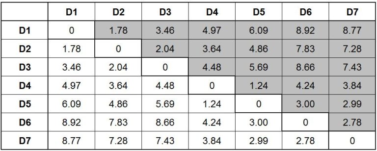
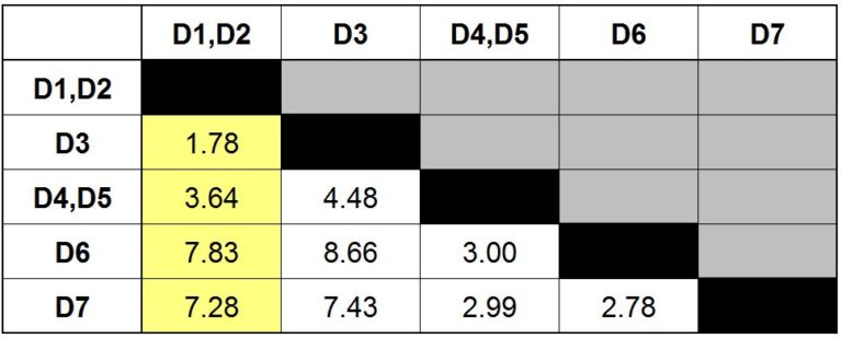
In this example, however, we will be creating clusters using the single linkage method only. Therefore, when we recalculate the distances, we come up with the following updated distance matrix.

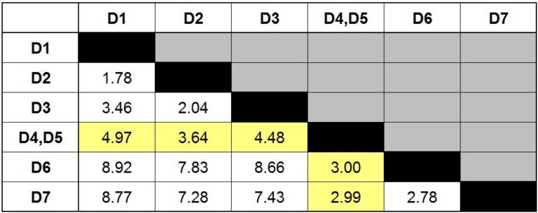
Notice that we don’t have any row or column for D4 and D5 anymore, and in place of that there is a new row, D4, D5. The updated distances are highlighted in yellow.

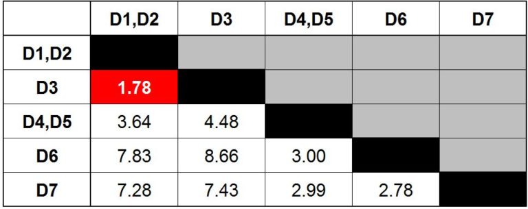
Step 4: From now on, we will simply repeat Step 2 and Step 3 until we are left with one cluster. We again look for the minimum value, which comes out to be 1.78, indicating that the new cluster that can be formed is by merging the data points D1 and D2.

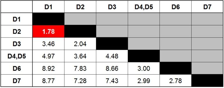
We now visualise this cluster on the graph and update the dendrogram.

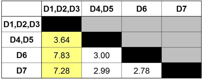
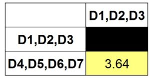
Step 5: Similar to what we did in Step 3, we again recalculate the distance, this time for cluster D1, D2, and come up with the following updated distance matrix.

Step 6: We repeat what we did in Step 2 and find the minimum value available in our distance matrix. The minimum value comes out to be 1.78, which indicates that we have to merge D3 into the cluster D1, D2.

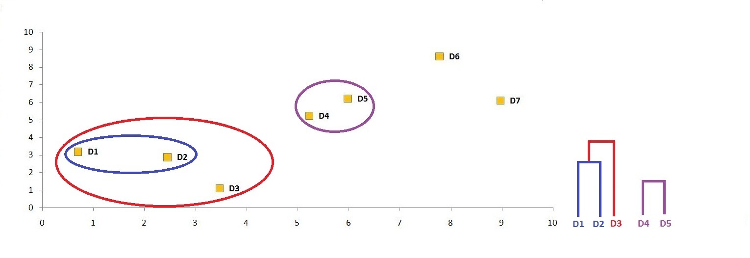
We visualise this new cluster on the graph and update the dendrogram.

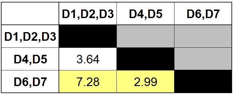
Step 7: Update the distance matrix using the single link method.

Step 8: Find the minimum distance in the matrix.

Merge the data points accordingly and form another cluster.

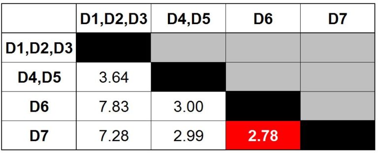
Step 9: Update the distance matrix using the single link method.

Step 10: Find the minimum distance between the clusters in the matrix.

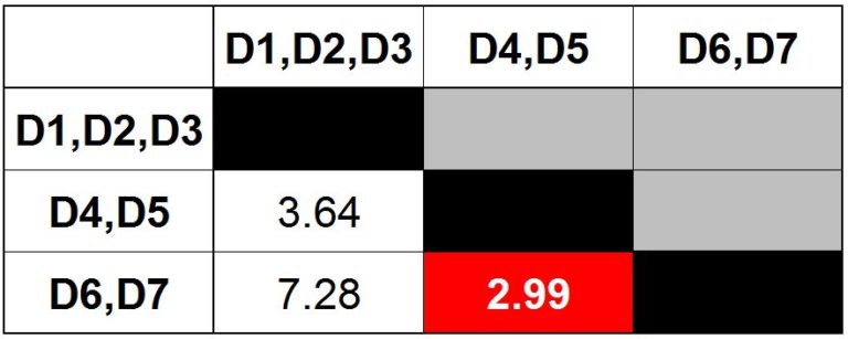
Merge the clusters to form another cluster.

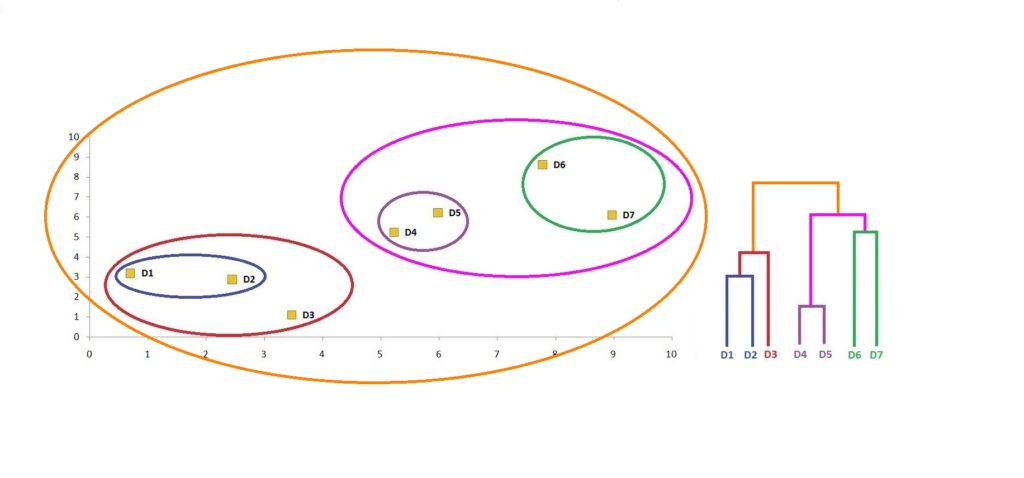
Step 11: As we are left with only two clusters, we can merge these two clusters.

Thus we are finally able to come up with a single cluster.

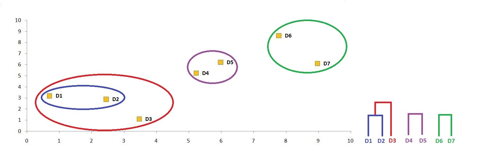
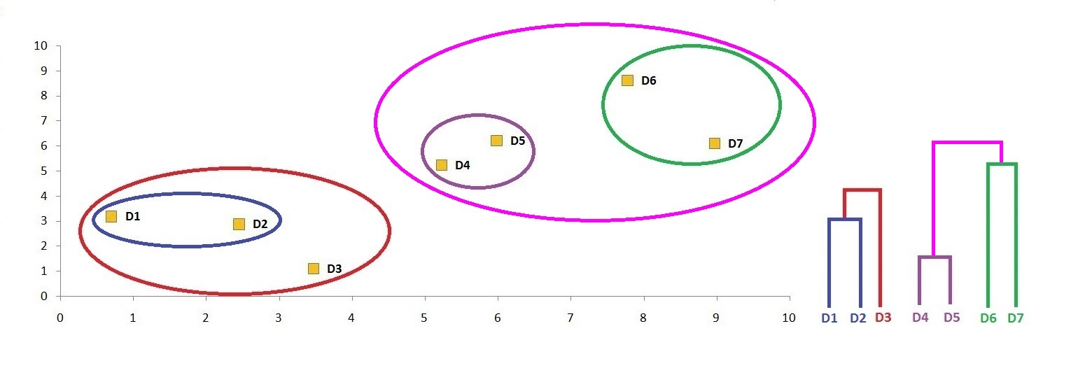
Step 12: We can now use the thresholds to come up with a number of clusters that might be meaningful to us. If we look at the graph, we can see that three clusters make the most sense: one cluster by combining the data points on the bottom left of the graph, a second by consolidating the data points in the middle, and a third cluster by merging the data points on the upper right of the graph. If we have to visualise this threshold on the dendrogram, then the cutoff point will be where we get the three-cluster solution.

Merits and Demerits of Hierarchical Clustering

Hierarchical clustering is a great method for clustering, as it is easy to understand and implement without requiring a predetermined number of clusters. It is also very easy to visualise, and it helps to make the clusters understandable visually through the help of dendrograms.

However, hierarchical clustering is sensitive to noise/outliers. Also, it requires standardization of data, as distance metrics such as Euclidean distance are used, which requires the data to be on the same scale for providing meaningful results. Also, the process is very complex, with the operation complexity being O(m² log m), where m is the number of observations.

Hierarchical clustering provides us with a dendrogram, which is a great way to visualise the clusters; however, it sometimes becomes difficult to identify the right number of clusters by using the dendrogram. Here we can either use a predetermined value of clusters, and when the hierarchical clustering algorithm reaches the predetermined number of clusters, we can stop the process. This, however, brings us back to K-Means clustering, where we were required to know the exact number of clusters to be found.

Therefore, the other method of finding the right number of clusters is by using cohesion, which indicates the goodness of the clusters. Thus, when using hierarchical clustering, if creating a cluster results in a low value of cohesion, we stop the process, and by doing so we are able to come up with the right number of clusters. There are multiple ways to define cohesion, such as by setting up the diameter of the cluster, where, when the newly formed clusters are more or less than the predetermined value of diameter, the algorithm stops creating clusters. Instead of diameter, we can also use radius, where the distance between the centroid of the cluster and the edge of the cluster is calculated. Another way is the density-based approach, where, rather than defining a threshold value of diameter or radius of the cluster, we define the minimum number of observations that should be there in the cluster, and when the algorithm is not able to create clusters with the predetermined number of observations, it stops creating any more clusters.

With all its advantages and disadvantages, hierarchical clustering continues to be one of the widely used clustering methods because of its more visual and easy-to-understand approach.