// clustering problems

K-Means

Among the most common methods of clustering is K-Means clustering. As mentioned at the beginning of this section, it is an unsupervised method of categorising data into different clusters, i.e. groups. The K here represents the number of groups that are to be found in the data. K-Means is a Hard and Flat clustering method, and as mentioned at the beginning of this section, what we mean by hard clustering is that every data point here is not present in multiple clusters, making the clusters unique. Thus here the clusters do not overlap each other. By saying that K-Means is a Flat clustering method, we mean that it is not hierarchical, and every cluster is not a part of some other cluster. Let us take an example to understand how K-Means works.

How the Algorithm Works

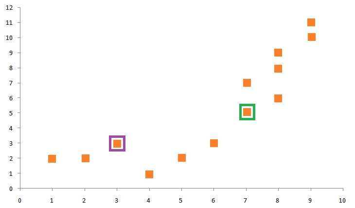
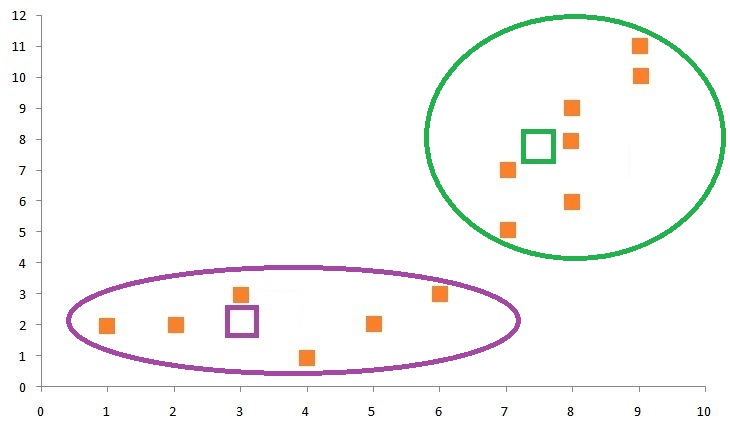
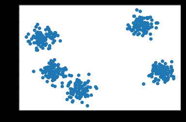
Suppose we have a dataset with two features. When plotted on a graph, we get the following figure:

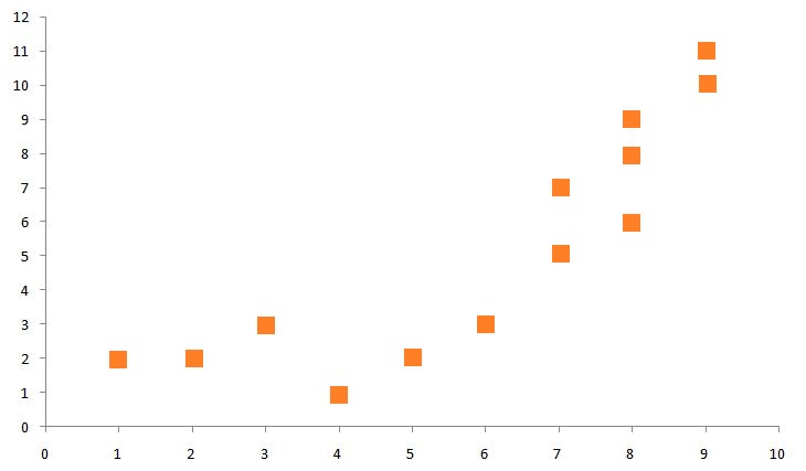
Scatter plot of a dataset with two features showing data points spread across two loose groupings

Now we first start by taking an arbitrary number of k. Let’s say we take k=2. Now to form two groups from the above set of data, the algorithm chooses two random points as the centroid and computes Euclidean distances from the centroid to all other data points. Let’s say that the centroid on the right has the label ‘1’ while the one on the left has the label ‘2’.

Two random data points selected as initial centroids, one on the left circled in purple and one on the right circled in green

The algorithm, after measuring the distances of all the data points from the centroid, associates each data point with a centroid based on its proximity.

Data points enclosed in two ovals, one purple and one green, showing each point assigned to its nearest centroid

K-Means algorithm works on iterations, as it now updates the centroids by taking the mean of all data points assigned to each centroid’s cluster.

We can see that now the centroid is in a different position. It repeats the above-mentioned process, again computes the mean, and updates the position of the centroid until no data point changes the cluster upon updating of the centroid. This is known as the point of convergence.

Thus K-Means is a very simple algorithm, unlike the other algorithms of supervised learning, where we had labels and updated the algorithm based on the error we got in the output.

Mathematical Calculation

To better understand the algorithm explained above, we can do some calculations and understand how Euclidean distance is calculated and centroids are updated to form clusters.

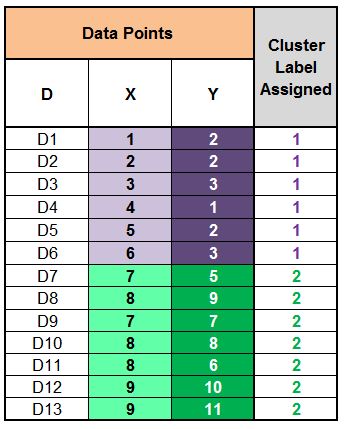
For example, we want to form two clusters (k=2) with a dataset having two features, X and Y, with 13 data points (samples).

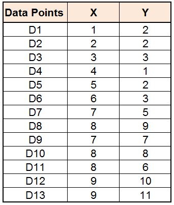
Table of 13 data points D1 through D13 each with an X and Y value

When plotted on x and y coordinates, we get the scatter plot we saw above.

Now we have to select random data points as the centroid. For example, we select Datapoint 3 as Centroid 1 (Cluster Label = 1) and Datapoint 7 as Centroid 2 (Cluster Label = 2). These two data points act as our initial random centroids.

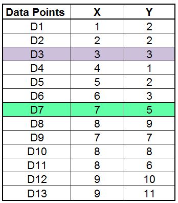
Table listing the 13 data points with D3 and D7 highlighted as the chosen initial centroids

We can also mark them on our graph to have a better understanding of where they lie.

Scatter plot with Datapoint 3 marked with a purple square outline and Datapoint 7 marked with a green square outline as the initial centroids

The second step is to calculate the distance from each of these two centroids to all the data points. We will here use the most common distance metric, the Euclidean distance, whose formula is:

Euclidean distance formula d equals square root of the sum of x2 minus x1 squared and y2 minus y1 squared

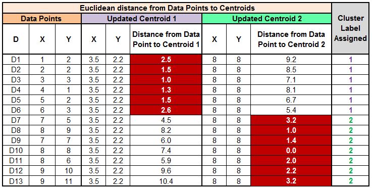
After calculating the Euclidean distance from each of the data points to the centroid, we come up with the following table:

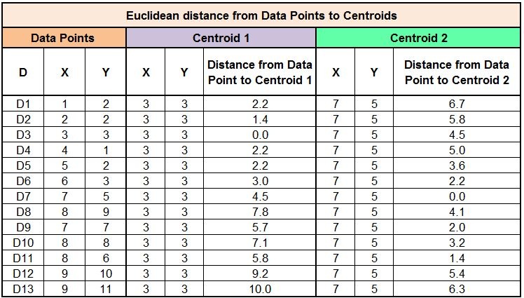
Table showing the Euclidean distance from each of the 13 data points to Centroid 1 at 3,3 and Centroid 2 at 7,5

We now have to compare the Euclidean distance between each data point and the two centroids. For example, for the first sample (D1), we can see that the distance between D1 and Centroid 1 is less (2.2) when compared to Centroid 2 (6.7). Therefore we can assign this data point to Centroid 1, i.e. Cluster Label = 1.

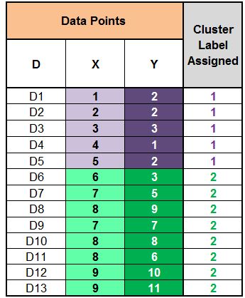
Similarly, we do this for all the samples and assign them to a cluster based on their proximity to the centroid.

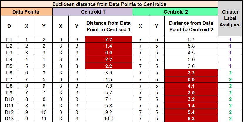
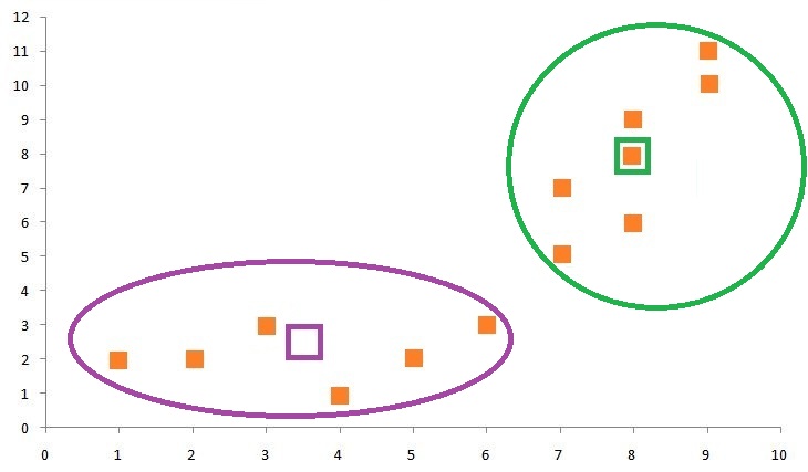
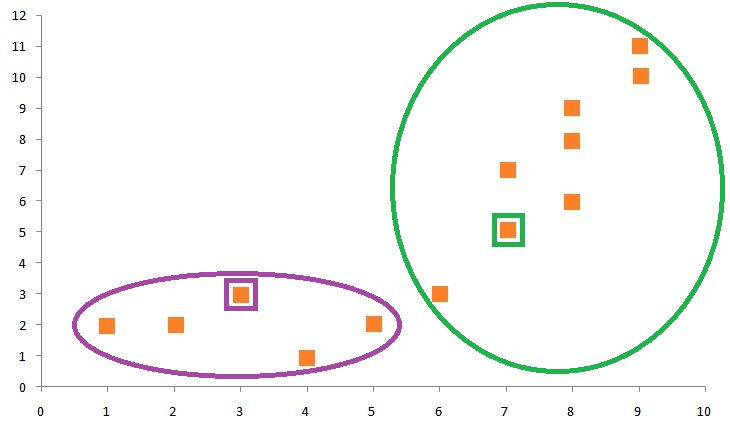
Distance table with the smaller of the two distances highlighted in red for each data point and the resulting cluster label assigned

If we form a cluster on the graph, we will see that the data points on the bottom left of the graph form a cluster (Cluster Label 1) and the data points on the top right form a cluster (Cluster Label 2).

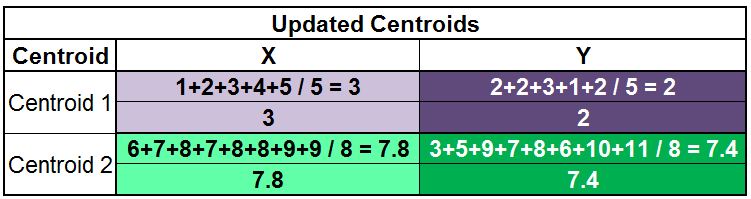
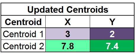
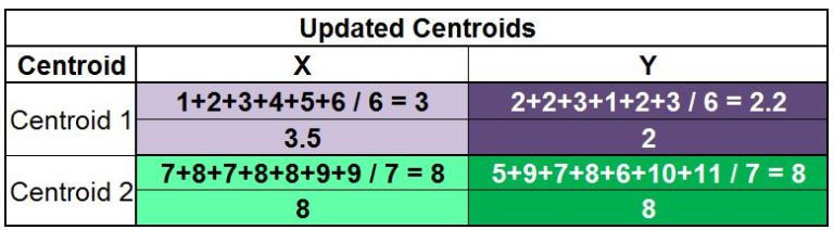
Scatter plot with a purple oval enclosing the bottom-left cluster and a green oval enclosing the top-right cluster

As mentioned above, we have to update the centroids, which we do by taking the mean of all data points assigned to each centroid’s cluster. Therefore, for finding the updated Centroid 1, we take the mean of all the data points that form Cluster 1. We do the same to find Centroid 2.

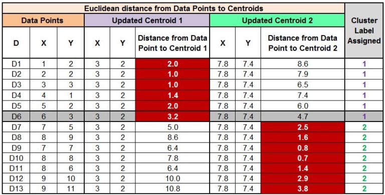
Table of the 13 data points colour-coded by their assigned cluster label, five points in cluster 1 and eight points in cluster 2

Calculation showing Centroid 1's X as the mean of 1,2,3,4,5 equal to 3 and Y as the mean of 2,2,3,1,2 equal to 2, with Centroid 2's X and Y means worked out from its eight assigned points

We again calculate the distance from each of these updated two centroids to all the data points and compare the distances to assign clusters to the data points. We find that the D6 datapoint, which was earlier classified as Cluster Label 1, now gets classified as Cluster Label 2.

Table showing the updated Centroid 1 at 3,2 and Centroid 2 at 7.8,7.4

Updated distance table showing D6 now closer to Centroid 2 than Centroid 1, with the smaller distance for D6 highlighted under Centroid 2

Scatter plot with the purple oval now excluding D6 and the green oval enclosing it along with the rest of the top-right cluster

As mentioned earlier, the algorithm keeps on reiterating the above process until it reaches the point of convergence, which means until no cluster labels are reassigned upon updating the centroids. If we again update the centroids and do the following calculations:

Table of the 13 data points with the cluster labels updated to reflect D6 moving into Cluster 2, six points in cluster 1 and seven points in cluster 2

Calculation showing Centroid 1's X and Y as the mean of the six points in cluster 1, and Centroid 2's X and Y as the mean of the seven points in cluster 2

We find that the new centroids come out to be Centroid 1 (3.5, 2.2) and Centroid 2 (8, 8).

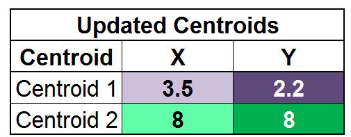
Table showing the final updated Centroid 1 at 3.5,2.2 and Centroid 2 at 8,8

When we calculate and compare the distances, we find that we have reached the point of convergence, as no cluster labels are updated anymore, and hence we can stop the process and come up with the final set of clusters.

Final distance table showing every data point's nearest centroid matches its existing cluster label, confirming convergence

Determining the Number of K

The single biggest parameter here is the value of k. There are multiple ways through which we can find the value of K.

Profiling Approach

This is a method where we identify the characteristics of each segment, and this method can be used if we have very good domain knowledge and have a lot of time at hand. Here we take multiple values of k. Then we analyse each of these clusters for various values of k, and the segment that provides us with the most meaningful results is chosen as the final value.

For example, we have a dataset, and we run the algorithm with k=3, k=4, k=5, k=6 and k=7, and we get the following results.

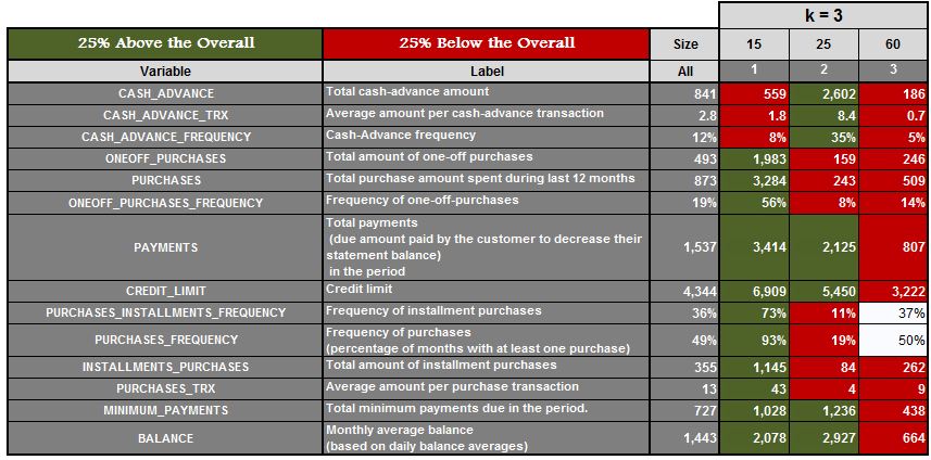
Table of cluster profiles for k equals 3, with each cluster's variables highlighted green where 25 percent above the overall mean and red where 25 percent below

Here for k=3, we get three clusters. We then find the mean of features for all these clusters and highlight the features which are 25% above the mean and 25% below the mean. We do the same for k=4, 5, 6 and 7.

Table of cluster profiles for k equals 4 with the same green and red highlighting scheme

Table of cluster profiles for k equals 5 with the same green and red highlighting scheme

Table of cluster profiles for k equals 6 with the same green and red highlighting scheme

Table of cluster profiles for k equals 7 with the same green and red highlighting scheme

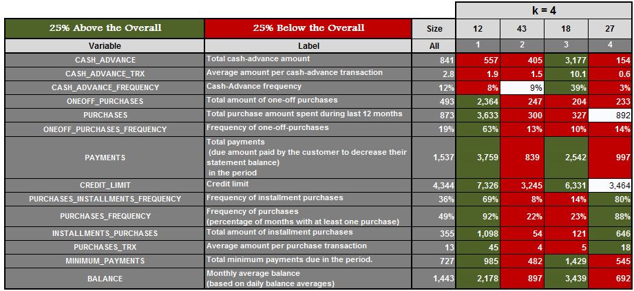
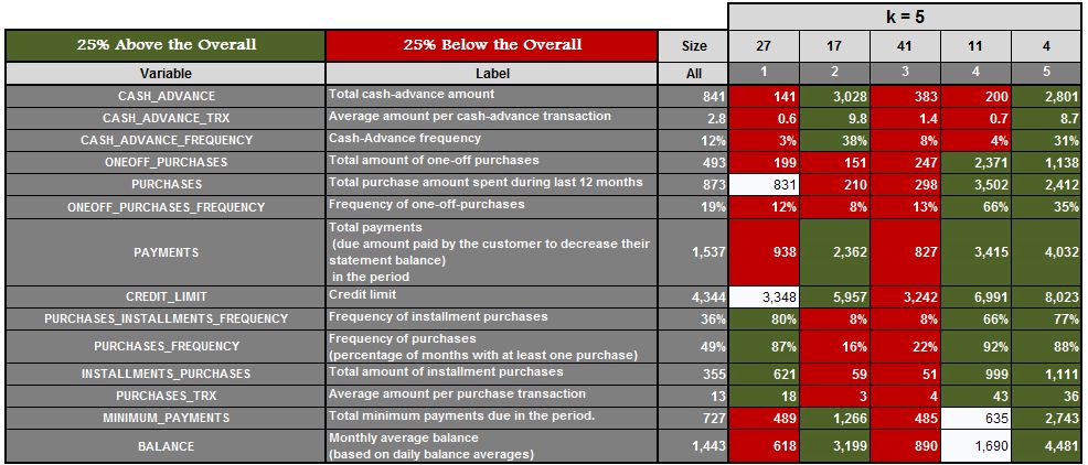
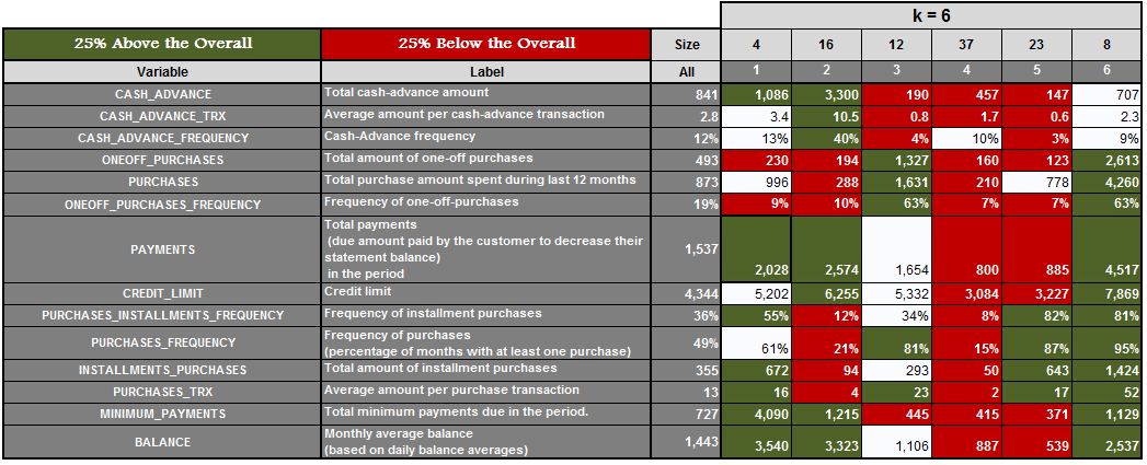
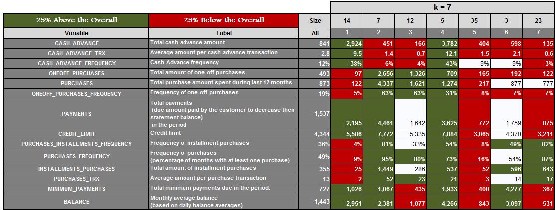
We can now analyse each of the clusters for each value of k and see which value of k provides us with the most meaningful clusters (in our example it came out to be k=5). This approach is, however, very time consuming and fails if we have no domain knowledge or have no idea of the range where the value of k should lie.

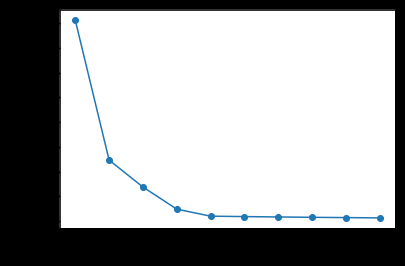
Scatter plot showing five distinct, well-separated clusters of points corresponding to the chosen k equals 5 result

Elbow Analysis

The other most famous approach is the Elbow Analysis. In this method, we compute the average distance of the data points from the centroid. With the increase in the number of centroids, the average distance between data points and their centroid decreases. We can use multiple values of k and plot them on a graph as shown below, and look for the value of k where the slope decreases and the average distance levels out.

Line plot of average distance to centroid against number of clusters, dropping steeply and then flattening out into an elbow shape

Other methods for validating the value of k include the Silhouette Coefficient, where the value of k that provides the largest coefficient is considered. Also, other metrics such as ANOVA, the SC Test, and Dendrograms can also be used.

Role of Seed

The objective of the algorithm is not to reduce the error (as we are in an unsupervised setup), but to minimize the aggregate distance from each centroid to the data points that are assigned to that centroid. Here we are concerned with intra-cluster distance (we do not care about the distance between the clusters). The problem with this clustering method is that we start by selecting the centroids randomly. Now we will converge no matter what random centroids we start with, but we converge to a local optimum, which means that if we start with different initial centroids, we will end up with a different result. To briefly understand this in the context of coding, we initiate the process (of the random selection of centroid) by providing a random seed in the code. Upon changing the seed, the value of k that we get from an elbow analysis can differ, which means that the initial random centroids affect the convergence. In a manual method, we can run the K-Means clustering for n number of k for m number of times, with each time having a different random seed, and then average the results of the elbow analysis to find the right number of k.

Pre-Processing Required for K-Means Clustering

Outlier Treatment

Like for all distance-based techniques, Outlier Treatment is required to be done on the data before using it for K-Means clustering. There are various outlier treatment methods that have been discussed in the Outlier Treatment article.

Missing Value Treatment

Many methods of handling missing values have been discussed in the Missing Value Treatment article.

Rescaling Data

As mentioned in Feature Scaling, distance-based algorithms need the data to be rescaled so that the metric makes sense to the algorithm.

Encoding

Also, the features need to be numerical, so one-hot encoding/dummy variable creation will be required if there are categorical variables in the data. This has been discussed in the Encoding article.

Dimensionality Reduction

There are various Dimensionality Reduction techniques, such as PCA, that can be applied to reduce the number of features which are unnecessary and can make the output of K-Means less meaningful.

K-Means is one of the most useful methods of clustering; however, it can suffer when the data is arranged in a particular way (such as half-moon-shaped datasets). Also, K-Means is heavily dependent on the predetermined number of k, and its results can be affected by the seed used for initialisation. Despite all these shortcomings, K-Means is one of the easiest clustering algorithms to understand and implement.