Clustering Problems in R

Clustering Problems are one of the most common problems solved in an Unsupervised Environment. Various clustering algorithms provide us with a method of grouping observation in such a way that the observations in the same group are similar to each other than those in other groups. As mentioned, this is an unsupervised modeling technique, as here we do not control how the clusters will be made. The only thing that we can control in this modeling is the number of clusters and the method deployed for clustering. Various clustering techniques have been explained under Clustering Problem in the Theory Section. In this blog, we will explore three clustering techniques using R: K-means, DBScan, Hierarchical Clustering.

Importing Dataset

To demonstrate various clustering algorithms in R, the Iris dataset will be used which has three classes in the dependent variable (three type of Iris flowers) and using this dataset clusters will be formed.

library(MASS)
iris_data <- iris
View(iris_data)

Clustering Algorithms

In this blog, we will be discussing three main ways to create clusters out of the Iris dataset, which are K-Means, DBSCAN, and Agglomerative Clustering aka Hierarchical Clustering.

K-Means Clustering

One of the most commonly used method of clustering, K-means clustering allows us to define the required number of clusters. To know about the workings of K-means refer to the blog: K-Means in the Theory Section.

Deciding Value of K

The most crucial aspect of K-Means clustering is deciding the value of K. We do this by performing elbow analysis. Refer to the K-Means Theory blog for more information on why and how this actually works. We first run K-means for the value of K from 1 to 11.

#Run the following command in the editor window for elbow method

wss <- sapply(1:11,
  function(k){kmeans(iris_data[,1:4], k,
    nstart=50,
    iter.max = 15)$tot.withinss})

We now plot the WCSS obtained from the above code. WCSS or within-cluster sum of squares is a measure of how internally coherent clusters are. K-Means tries to minimize this criterion.

> plot(1:11, wss,type="b", pch = 19, frame = FALSE,xlab="Number of clusters K",
+      ylab="Total within-clusters sum of squares")

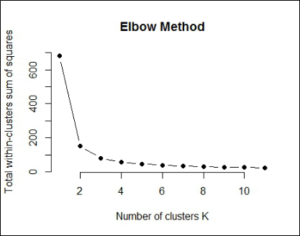
In the elbow graph, we look for the points where the drop falls and the line smoothens out. In the above graph, this happens for k=3. Another way of understanding this is that we note the point at which the WCSS is less and try to find the number of clusters for our dataset. We see that at the number of clusters = 3, WCSS is less than 100, which is good for us. So we take k =3.

Running K-Means Model

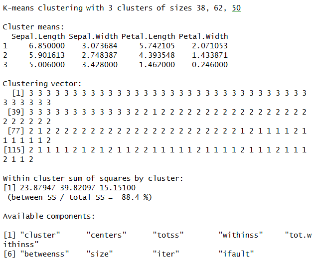
We now run K-Means clustering for obtaining a 3 cluster solution.

clust_kmeans <- kmeans(iris_data[,1:4],3,nstart = 20)
clust_kmeans

We now also create a table from the above output.

table(clust_kmeans$cluster,iris_data$Species)

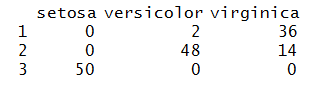
When compared to the original classes we find that the observations of the class label Iris-setosa has been correctly formed into a separate well-defined cluster, however, for the other two classes, clusters are not as correct. This is mainly because, in the original dataset, these two class labels were overlapping each other which makes it difficult for the clustering algorithm as it works best for clear neat separate observations. Still, the clusters have been formed more or less correctly.

DBScan

DBScan, an acronym for Density-Based Spatial Clustering of Applications with Noise is a clustering algorithm. It makes clusters based on their densities. It identifies observations in the low-density region as outliers.

Importing Library

We import dbscan to run a DBScan model.

install.packages("dbscan")
library(dbscan)

Transforming Data

Transforming the iris dataset with four features to matrix form.

iris_mat <- as.matrix(iris_data[,1:4])

Initialize Model

We now initialize the DBScan Model with eps (epsilon) = 0.42

db <- dbscan(iris_mat,eps = 0.42)
db

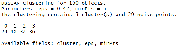
We can see the cluster labels assigned to various data points. Here, the 0s will be the outliers.

db$cluster

Hierarchical Clustering

Hierarchical Clustering can be of two types - Agglomerative and Divisive. In this blog post, we will explore Agglomerative Clustering which is a method of clustering which builds a hierarchy of clusters by merging together small clusters. To know more about Hierarchical Clustering refer to the blog Hierarchical Clustering under the Theory Section.

Initializing Hierarchical Clustering Algorithm

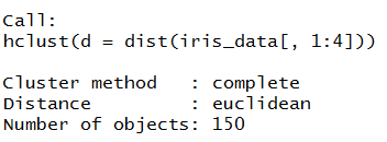
We will be using hclust function to perform hierarchical clustering.

clusters <- hclust(dist(iris_data[,1:4]))
clusters

Plotting of Dendrogram

We make use of dendrogram to decide the number of clusters required for our dataset. A dendrogram is a tree diagram which illustrates the arrangement of clusters.

plot(clusters)

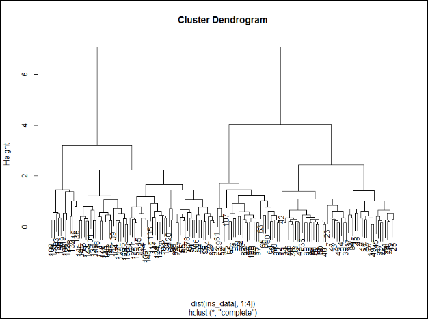
Building an Agglomerative Clustering Model

We analyse the above-created dendrogram and decide that we will be making 3 clusters for this dataset.

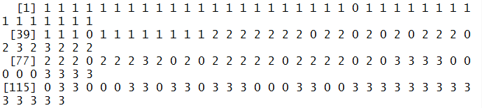
clusters1 = cutree(clusters, 3)
clusters1

We can compute a table showing the number of data points assigned to each cluster label.

table(clusters1, iris_data$Species)

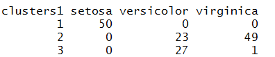
Here also we found that Iris-setosa has been clearly formed into separate cluster while the other clusters overlap each other.

In this blog post, we explored the application of three different clustering algorithms in R. All these algorithms have their own style of functioning and should be used when trying to solve clustering problems.