// important concepts

Hypothesis Testing

Hypothesis Testing is one of the most crucial aspects of the Inferential Statistics. As discussed in the ‘Descriptive Statistics’ section, numerous descriptive statistics are used for nothing but to describe the data, however through inferential statistics, we try to draw some conclusion and through hypothesis testing we try to determine that whether a phenomenon seen in a sample of population actually occurs in the population also and if it does or doesn’t, how sure can we be of either of the statement or if we try to compare means and create a hypothesis, how sure can we be about this hypothesis, for all this we can perform hypothesis testing so that we can reject or accept our hypothesis. Here hypothesis is nothing but a predictive statement that relates an independent variable to a dependent variable. There are various kinds of hypothesis testing for different scenarios. Some of the most important hypothesis tests are shown below.

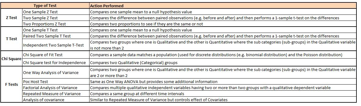Z Test, T Test, Chi Square, F Tests) and the action each one performs" />

Such Hypothesis tests are very useful as they provide clear and precise answers to our specific questions.

Null and Alternative Hypothesis

Every Hypothesis testing is done to either reject or accept a Null Hypothesis.

Null Hypothesis

The definition of a Null Hypothesis can vary for each type of a Hypothesis Test and also depends upon the problem at hand, but more or less the Null Hypothesis generally states that there is an absence of effect, i.e. for example if we are comparing a sample mean with the population mean, the null hypothesis will be that the two means are equal to each other.

H0: μ = x̄

Alternative Hypothesis

Alternative Hypothesis is the opposite of Null Hypothesis and states that the sample mean can be larger or smaller than the population mean, or to put it simply, the population mean is not equal to sample mean.

H1: μ ≠ x̄

Two-Tailed, One-Tailed Hypothesis

Two-Tailed

Sometimes, the alternative hypothesis merely states that the sample mean is not equal to the population mean. This is called a Non-Directional aka Two-Tailed Test because here we do not state a particular ‘direction’ for the hypothesis. Therefore the alternative hypothesis is rejected if the sample mean is not equal to the Population mean because of the sample mean either being too large or too small from the population mean. Such an Alternative Hypothesis is stated when researchers are not aware if the outcome will be negative or positive.

One-Tailed

On the other hand, Directional aka One-Tailed Hypothesis is where we set the alternative hypothesis of the possibility we are interested in for example if we are only interested in finding if the sample mean is larger than the population mean or not. Here a smaller value or say a decrease in the sample mean is of no use to us. Therefore we set our Alternative Hypothesis as

H1: μ < x̄

Types of Error

There are two types of errors that a researcher can commit while doing a hypothesis test- Type I and Type II.

Type I Error

Rejecting Null Hypothesis when it should have been Accepted.

Type II Error

Accepting Null Hypothesis when it should have been Rejected.

Any of such mistakes can cause very wrong interpretation of the data and such mistakes should be avoided at any cost.

P Value, Significance Level and Confidence Level

P Value

We use the p-value to either reject or accept a null hypothesis. On the basis of p-value, we decide how significant the ‘change’ is. It is the most basic and crucial aspect of any kind of Hypothesis Test and should be clearly understood to avoid the Type I and Type II mistakes. In simple terms, the p-value is the

Probability of finding the observed or more extreme results when the null hypothesis is true- Probability for a given statistical model that, when the null hypothesis is true the statistical summary (such as the sample mean difference between two compared groups) would be the same as or of greater magnitude than the actual observed results.

Significance Level

The Significance Level (symbolised as α (alpha)) is used to refer to a pre-chosen probability which we will use to reject or accept the null hypothesis. We calculate the p-value and on the basis of the “cut off” or Significance level we accept or reject the null hypothesis. For example, our Significance Level is 5%. What we mean by setting a 5% Significance level is that the random chance of getting our tested value (e.g. a sample mean) is less than 5%. Here if the p-value comes out to be eg 0.04 (4%) then we can say that the chance of getting our tested number (eg. sample mean) randomly is less than 4% and we say that the number we got is not due to chance as the probability of getting such a number by chance is as low as 4% and as per our significance level, if the probability of getting a number by chance is less than 5%, we would conclude that the change in our sample mean is statistically significant. However, if we would have set our significance level at 1% then the sample p-value would have made us conclude that the number we have got is by chance and is due to random sampling. Here for our sample mean to be significant, the p-value should be less than 0.01 i.e. less than 1%. Therefore the Significance level is very subjective and varies as per the requirements of the business scenario or the domain in question.

Confidence level

Confidence level is simply 1-Significance level i.e. if our significance level is set to 5% then our confidence level is 95% and if our p-value comes out to be 0.04, then we can be 96% confident that our sample mean is not due to randomness or by chance but indicate an actual change in the mean.

In general, the significance level is set to 5%. And the p-value (P) generally means-

• P > 0.05 - statistically insignificant (more than 1 in 20 chance of being wrong)
• P < 0.05 - statistically significant (less than 1 in 20 chance of being wrong)
• P < 0.01 - statistically significant (less than 1 in 100 chance of being wrong)
• P < 0.001 - statistically highly significant (less than one in a thousand chance of being wrong)

To use the p-value for Accepting or Rejecting the Null Hypothesis, it is important to remember that if our p-value is less than the chosen significance level then we reject the null hypothesis i.e. accept that our sample value (e.g. sample mean) gives strong evidence to support the alternative hypothesis.

A Cheat way of remembering this is to remember phrases. A phrase that can be used is-

“If P is low Null will go, if P is high then Null will decide”

It is a very intuitive way of remembering but sometimes helps. So if the set significance level at 5% and the p is low (lower than the 0.05 mark) then we reject the Null Hypothesis (Null will go) and if our p-value is high (higher than the 0.05 mark) then we accept the Null Hypothesis (Null will decide and will be used to draw the inference).

Examples

To explain p-value, Significance and Confidence Level, 3 examples are used below wherein Example 1 and 2 the Alternative Hypothesis will be Directional while in Example 3, the Alternative Hypothesis will be Non-Directional.

Example 1

Firstly, understand the p-value in layman terms. For example, we have known that a company XABZ Corp. does campus recruitment and hire students who on average have scored 70% in their graduation. They are known to have a standard deviation of 8% marks. Here our Population mean is 70 while our standard deviation of population means that the company hired students who scored marks more than 70% and also hired students who scored marks less than average and this variation in marks is indicated by the standard deviation of population which is 8% i.e. the swings of marks was of 8 percent. In theory, any score that lies below this standard deviation will be rejected. Now this year 100 students got selected who on average scored 68% marks in their graduation. Now the question is, has the company started hiring students who have scored marks less than the earlier said average. We set our Null Hypothesis that states that there is an absence of an effect, i.e. if comparing a sample mean with a population mean, the null hypothesis is that the two means are equal to each other. Here the Null Hypothesis is that there is no change and the change of marks reflected in the sample is simply due to chance. So our Null Hypothesis is - H0: μ = x̄. Here the Alternative Hypothesis is Directional aka One-Tailed Hypothesis where we state that the sample mean (68% graduation marks) is significantly less than the population mean (70% marks) i.e. H1: μ > x̄. Here (as in Directional aka One Tail Hypothesis). Here an increase in the sample mean (or graduation score) is of no use to us as we know that higher marks will obviously mean better chances of getting into a company, but we are mainly concerned about the lower side and want to know if the criteria is somehow relaxed by the company.

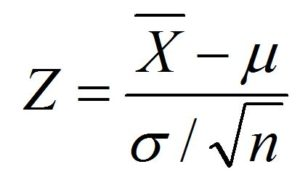
Here we know the population mean and its standard deviation and we presume that the population distribution is normal. Here we will do a Hypothesis Testing by doing a Z-Test (as Standard Deviation of the Population distribution is available to us and is presumably normally distributed)

z = x - μ / σ

z = 68-70/8 ÷ √(100)

z = -2.5

Here the z value is negative as the value we are trying to test (this year’s sample mean score which is 68%) is less than the average (70%).

To understand now what p-value is, we should be able to place our z value on the distribution. To do this, we will use the Table of Standard Normal Probabilities for Negative Z-scores and calculate the value it returns which will be the p-value. This p-value will let us know about the area to the left of the z score which is the probability of how strongly we are rejecting or accepting the null hypothesis.

In our example when we compute the p-value from the table for the z value of -2.5, it comes out to be 0.0062.

Now before accepting or rejecting the null hypothesis we decide our significance level to be at 5%. As our p-value is lower than our significance level, we reject our Null Hypothesis and state that the criteria of selection have changed and students with lower marks are now also able to crack the recruitment process and we can be 99.38% confident about our alternative hypothesis. (1-Significance is our confidence for the alternative hypothesis).

The Confidence Level and p-value can often be confusing and one might get confused what the confidence is about. To clear any doubt, suppose the average marks of the students recruited by the company were 72.5. Now if we would have concluded with the same Null and Alternative Hypothesis, our z values would have been 3.12 (72.5-70/8÷ √(100)). Here the p-value would have come out to be 0.9991. Now as the p-value is higher than our set 5% significance level, we would have accepted our Null Hypothesis which states that no change has been there in the recruitment process and would have been less than 0.09% confident about the hypothesis that the company has reduced the marks required to make it in the company.

Example 2

MedecialLabs001 produces a pill, “Pill O”, that can control a fever in 1.2 hours. Now a team of medical scientists come up with a “Pill N” that has a new chemical formula and tested it on 100 human beings and on average it controlled fever in 1.05 hours with a standard deviation of 0.5 hours. Now the head of the company needs to decide whether to launch “Pill N” in place of “Pill O” and for that, he needs to be sure that the new medicine is actually effective and the change in mean is not due to chance.

Here as we don’t know the standard deviation of the population and only know the sample standard deviation we will do a One-Sample T-Test for our Hypothesis Testing and will compute a t-score to find the p-value.

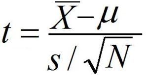
Here we first decide our Null Hypothesis which will state that there is no difference between the population and the sample mean i.e. H0: μ = x̄. Our Alternative Hypothesis, however, will state that the sample mean (time taken to control fever by “Pill N”) is less than the population mean (1.2 hours) i.e. H1: μ > x̄. Here (as in Directional aka One Tail Hypothesis), a bigger value or say an increase in the sample mean is of no use to us as we know that higher time will obviously mean that the new drug is no better than the previous one, rather we are more interested in knowing if the new drug’s mean is lesser then the population mean or not.

Now we set our significance level at 5%.

We compute the t value by subtracting the population mean from the sample mean and dividing it by the Standard Error of mean. Here the standard error of mean is calculated by dividing the standard deviation of the population by the square root of the number of samples.

The t value comes out to be -3. The t-distribution table only shows us the p values for positive t value. To know the p-value of a negative t value we simply find the p-value of its corresponding positive number. We calculate degrees of freedom which in this case will be N-1 i.e. 100-1=99. When we look at the t-Table it turns out that the t value is significant and the difference between the population and sample mean can be considered to be extremely statistically significant. The critical t value comes out to be 1.660 with the probability of P(μ = x̄) = 0.00341551. Thus we reject our Null Hypothesis and State that the difference between the population mean and sample mean is not by chance but rather is statistically significant.

It has been mentioned in earlier blogs that if the sample size is large enough, say more than 30, then the difference between a Z-test and t-Test is not much. Here we can prove this. We presume that if the population standard deviation has been 0.5 hrs then we would have been able to perform a Z test. The Z value from such a Z Test would have also been an obvious -3.

Now if we look at the z table and find the p-value, it comes out to be 0.0013. Here also as the P value is low and we reject the Null Hypothesis and can be 99.87% confident that our Alternative Hypothesis is correct.

Example 3

The average income of a graduate in city ‘X’ has traditionally been said to at 45,000 with a standard deviation of 3,000. A survey is conducted with 120 working graduates where the average income came out to be 45,500. Has the average income for graduates changed or is the change in the income due to random chance.

Here we set our Null Hypothesis to be that there has been no change in the sample mean and the population mean, however here our Alternative Hypothesis simply states that the sample mean is not equal to the population mean i.e. H1: μ ≠ x̄.

Now here we will use a Z-test as the standard deviation of the population is available and the sample distribution will be normally distributed (as the sample size is more than 30).

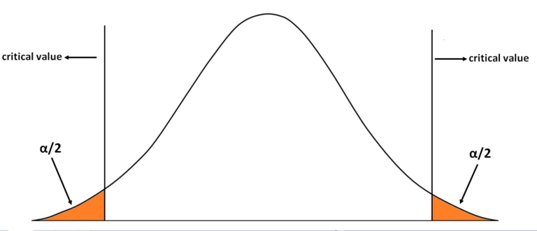
However interestingly, whatever the p-value we get from the z table, we will double it and then compare it to our pre-determined significance level which will be at a level of 5%. This is done because unlike a One-tailed Alternative Hypothesis where we look at the data under the curve either to the left or to the right side of our sample mean, in a Two-Tailed Alternative Hypothesis, we consider both the extremes. To explain this further lets first calculate the z-value.

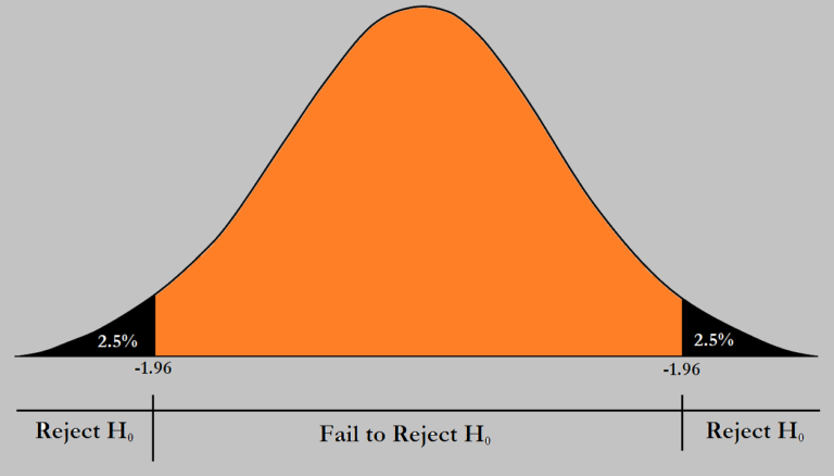
Here the z-value will be 1.82 (45,000-45,500/3,000 ÷ √(120)). Now if we understand this graphically, earlier when our significance level was set at 5% then what we meant was that the left most or right most 5% of the curve will be our reject region (depending upon the type of Alternative hypotheses) and if our p-value lies there then we can reject our Null Hypothesis. Here, however, our Acceptance Region will be the middle and the reject region of 5% will be divided among both the sides, providing 2.5% to each of the sides of the distribution.

Now we use the Table of Standard Probabilities for negative z score to find the p-value for the left slide of the curve. For this let’s consider our z value to be negative. So the p-value for -1.82 comes out to be 0.0344. It is important to remember that we have to find the p-value for both the sides and for that we simply multiply our current p-value by 2 i.e. 0.0344 × 2 = 0.0688. Here our p-value is larger than our hypothesis and thus we can accept our Null Hypothesis which states that there has not been any statistically significant change in the income, and the change in the sample mean was due to chance.

To understand this more intuitively, we find that the average salary is 45,000 and even when the standard deviation is 1.82 i.e. the average salary deviated by 1.82 standard deviations, it doesn’t include the 45,500 figure. To get this value, it has to deviate beyond this standard deviation. We have set our significance level at 5%, i.e. if such a value can be found in less than 20, then it is not by chance, however, if such a value can be found more than 1 in twenty then it is probably due to chance. Here our p-value comes out to be more than set 5% (i.e. more than 0.05) and thus we state that the increase in our sample mean was probably due to chance.

Effect Size

So far we have followed certain steps where we find the difference between the sample statistic and the population parameter and divide this difference by the standard error and determine the probability of getting this ratio by chance (random sampling error).

However, there is a flaw in this process, which is that the denominator plays a major role where the standard error present in all the denominators becomes smaller when the sample size is large and smaller the standard error, higher the chances of considering it statistically significant and because of this, a very small difference in the sample statistic and population parameter can be considered statistically significant (if the sample size is large enough).

Thus for instance, if there is a large difference between the sample mean and the population mean but the sample size is of 20 then it may not be considered statistically significant however the same difference will be considered significant if the sample size is of 2000.

Thus researchers nowadays consider both- The statistical significance as well as the effect size.

Confidence Interval and Point Estimate

These two types of estimators- Confidence Interval and Point Estimate which are two types of inferential statistics that provide us with insights that are useful for modeling and predictive analysis.

Confidence Interval

You must have seen the example of confidence intervals in your day to day lives. It is among the commonly used inferential statistics. Confidence Intervals are used by researchers when they don’t know the actual population parameter (population mean). Thus we calculate the confidence interval that provides us with a range of values of which we are confident to a certain degree that the range contains the population mean. To further understand this, consider the below examples.

Examples

Below are some examples that will help in understanding how Confidence Interval works.

Example 1

Suppose the sample mean is 10. Standard Deviation of the sample is 2. Degrees of freedom is infinity (i.e. number of samples are a lot). We want a range of population mean at a 95% and 99% confidence level.

The formula to calculate this will be

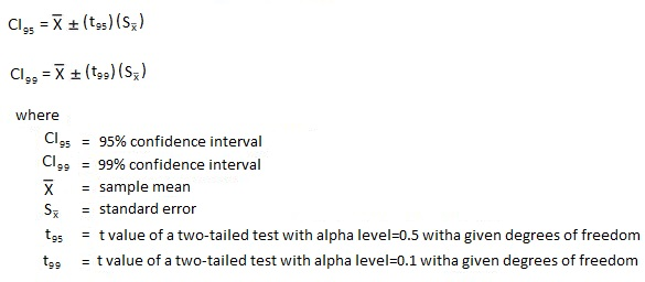
Now we look at the t table and for df = ∞ and α = .05, we find t95 = 1.96.

CI95 = 10 ± (1.96)(.06)

CI95 = 10 ± .12

CI95 = 9.88, 10.12

Thus our range for the population mean comes out to be 9.88 to 10.12 at 95% confidence.

For 99%, we will see that the range increases i.e. for being more sure about our outcome

CI99 = 10 ± (2.576)(.06)

CI99 = 10 ± .15

CI99 = 9.85, 10.15

Thus our range for the population mean comes out to be 9.85 to 10.15 at 99% confidence.

(Notice how the minimum value gets even lower and the higher value is pushed further high)

Example 2

The sample size is 36 (N=36), the mean of the sample is 25.5. What is the population mean?

Here we can use a simple formula-

μ = x ± SE

μ = 25.5 ± 3.6 ÷ √(36)

μ = 25.5 ± 0.6

μ = 24.9 to 26.1

Here the confidence level is at 1 std and we know that for a normal distribution, the area under the curve within one standard deviation is about 68.3%, so we can be roughly 68% confident about this value. To have a 95% confidence i.e. 2 std we simply multiply the standard error by 2.

μ = 25.5 ± 0.6 × 2

μ = 25.5 ± 1.2

μ = 24.3 to 26.7

Point Estimate

Point estimate is where we try to estimate a statistic pinpoint rather than providing a range.

For Example, the sample variance is an example of point estimate and in a way, any statistic can be a point estimate. An example of that can be of estimating the average rainfall in Mumbai.

With the knowledge of how a hypothesis testing works, we can now understand the various statistical tests that can be used to test a hypothesis and draw inferences from the sample. The various statistical tests mentioned in the next few blogs are t-Tests, F-Tests, chi-square.