// feature selection

Embedded Methods

In embedded methods, we use modeling algorithms that use the coefficients of features to reduce them. Embedded Methods are among the most sophisticated feature selection methods, as they in a way combine the qualities of Filter and Wrapper methods.

Process of Embedded Methods

For Embedded Methods, we need to have the features on the same scale. Then we can simply presume that the features that have the highest coefficients in the model are the ones that are important and influence our dependent variable, and the features that are not correlated to the output variable have coefficient values close to zero or even zero. However, it is not as easy as it sounds, because every feature influences the output variable, and if the number of features is too large, then the size of the coefficients shoots up, making it difficult to decide which features are important and which are not.

This leads us to use regularized models that have a built-in function to control the size of these coefficients.

It is advised to read Linear Regression to understand the content mentioned below.

We can use two types of Embedded Methods: Lasso Regression (uses L1 regularization) and Ridge Regression (uses L2 regularization), which are regularized linear models that can be used for feature selection.

Ridge Regression

Ridge Regression can be used to create a regularized model where constraints are put in the algorithm to penalize the coefficients for being too large, thus preventing the model from becoming too complex and causing overfitting. In very simple terms, it adds a penalty α‖w‖ to the equation, where w is the vector of model coefficients, ‖·‖ is the L2 norm, and α is a tunable free parameter, making the whole equation look like the one below.

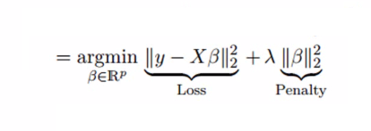
Here the first component is the least squares term (loss function), and the second is the penalty. In Ridge Regression, L2 regularization is done, which adds a penalty equivalent to the square of the magnitude of the coefficients. Thus, under Ridge Regression, an L2 norm penalty, which is α∑w², is added to the loss function, thereby penalizing the betas. Here, as the coefficients are squared in the penalty component, it has a different effect than an L1 norm, which we use in Lasso Regression (discussed below). The choice between Ridge and Lasso, and the Elastic Net that blends the two, is set by a separate mixing parameter (often called the L1 ratio): a value of 0 gives pure Ridge, 1 gives pure Lasso, and anything in between gives Elastic Net. Note that this mixing parameter is different from the penalty strength described above - confusingly, some libraries also call one of these ‘alpha’. In R’s glmnet, alpha is the mixing parameter, whereas in Python’s scikit-learn alpha is the penalty strength and the mix is set by a parameter called l1_ratio.

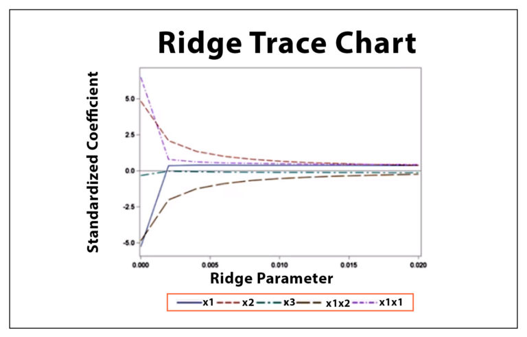
This leaves us with the most crucial aspect, which is deciding the value of the tunable parameter lambda. If we use a very low lambda value, then the output will be the same as OLS Regression, and thus not much generalization will take place; however, if we take too big a value for lambda, it will generalize too much, pulling down the coefficients of too many features towards extreme minimum values (i.e. towards 0). Statisticians use methods such as the Ridge Trace, which is a plot that shows ridge regression coefficients as a function of lambda, and we select the value of lambda where the coefficients stabilize. We can use methods such as cross-validation along with grid search to find the best value of lambda for our model.

Ridge uses L2 regularization, forcing coefficient values to be spread out more equally and not shrinking any coefficient to the extent that it becomes 0; however, L1 regularization forces the coefficients of the less important features to be zero, and this leads us to Lasso Regression.

Note: Ridge Regression may or may not be considered a Feature Selection method, as it only reduces the size of coefficients and, unlike Lasso, doesn’t make any variable obsolete, which can properly be called a Feature Selection method.

Lasso Regression

Lasso works the same way as Ridge but performs L1 regularization, which adds a penalty α∑|w| to the loss function, thereby adding a penalty equivalent to the absolute value of the magnitude of the coefficients, rather than the square of the coefficients (used in L2), making the weak features have zero as their coefficients. In a way, by using L1 regularization, Lasso performs automatic feature selection, where features with 0 as the value of their coefficients are dropped. Again, the value of lambda is important, as if the value is too large, it ends up dropping a lot of variables (by causing coefficients that are a bit small to become 0), making the model too generalized and causing it to underfit.

By using the correct value of lambda, we can have a sparse output where certain unimportant features are given 0 as coefficients, and these variables can be dropped, while variables with non-zero coefficients can be selected, thus facilitating feature selection for modeling.

Thus, these regularized linear models can be used to find the correct relationship shared between the independent and dependent variables by regularizing the independent variable’s coefficients. They help us curb the menace of multicollinearity. Applying regularization to certain regression models can be problematic where the independent features are non-linearly related to the dependent variable. To counter this problem, we can transform the features so that linear models such as Ridge and Lasso can still be applicable, such as by using polynomial basis functions with linear regression, where such transformed features allow the linear model to find the polynomial or non-linear relationships in the data.