// model evaluation

Classification Models

Various model evaluation techniques can be used under the supervised learning setup that help us find the performance of the model. A very simple method to evaluate a model is by finding the accuracy, which is the difference between the predicted and actual values, and when working with classification models, by accuracy we mean the count of the correct predictions of the class labels. However it is not a perfect method and can lead to poor decision making. Therefore we need other measures to evaluate the various models, and picking the right measure of evaluation is crucial in selecting and distinguishing the right model from other models.

To understand the various metrics that can be used to evaluate a classification problem, we first need to understand what we mean by a Base Rate Model. For example, we have a dataset with 100 records where 90 records belong to class label '0' while the remaining 10 observations belong to class label '1'. As the frequency of the class label '0' is higher than class label '1', a model which predicts all observations to have the class label '0' will have an accuracy of as high as 90%. Therefore the accuracy here provides us with little information on how the model is actually performing. It is important for our model to have accuracy at least more than 90%, because a model that simply predicts the most frequent class already has an accuracy of 90%. This limitation of accuracy calls for more complex measures of evaluation.

Confusion Matrix

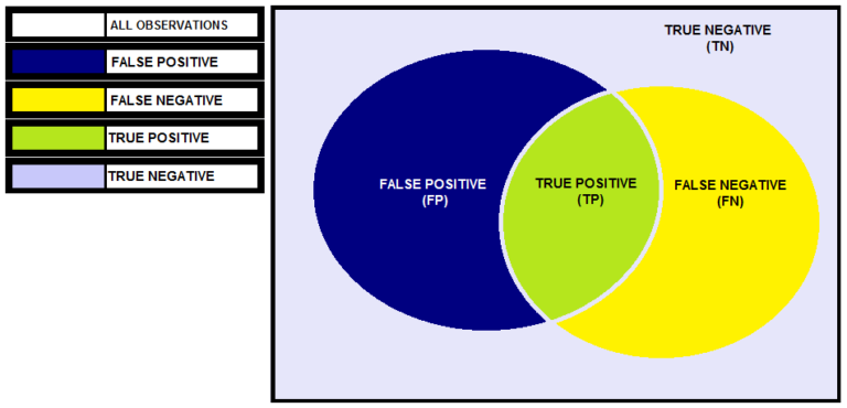
For example, we have a dataset having class labels 0 and 1, where 0 stands for 'Non-Defaulters' while 1 stands for 'Defaulters'. We build a logistic regression model to predict the class label 1. Below is a Venn diagram where all the observations are in the square box. All the observations that were predicted as 1 by the model are represented by the Blue Circle. All the observations that were actually 1 are represented by the Yellow Circle. The common area of these two circles is denoted in green and contains the observations that were correctly predicted by the model, called True Positives. False Positive observations are those that were incorrectly predicted as 1 by our model, while False Negative observations are those that were incorrectly predicted as having the class label '0' by our model. The remaining observations are the True Negatives, which are those that were correctly predicted as having the class label '0' by the logistic regression model.

Rather than a Venn diagram, we can come up with a confusion matrix to show all these observations. For a two-class classification problem, the confusion matrix will have two rows and two columns, where the rows represent the predicted values whereas the columns represent the actual values. Our objective is to minimize the False Positives and False Negatives and maximise the True Positives and True Negatives, thus we want to maximise the diagonal values.

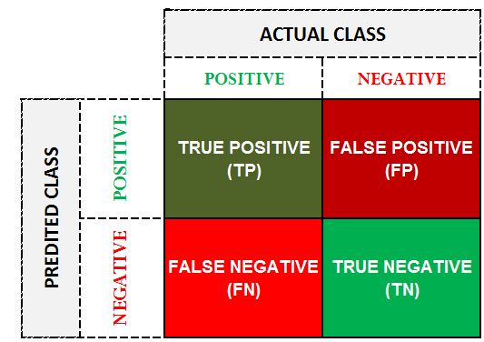
Positive (1) - Defaulter; Negative (0) - Non-Defaulter.

True Positive - Model predicted 'Defaulter' and the observation was actually 'Defaulter'. True Negative - Model predicted 'Non-Defaulter' and the observation was actually 'Non-Defaulter'. False Positive - Model predicted 'Defaulter' and the observation was actually 'Non-Defaulter' (Type I Error). False Negative - Model predicted 'Non-Defaulter' and the observation was actually 'Defaulter' (Type II Error).

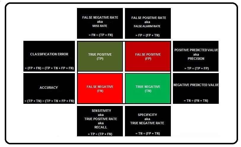
The real power of the confusion matrix lies in the various metrics that can be calculated from it. The most basic measures involve Classification Error and Accuracy.

Classification Error

The formula for Classification Error is (FP + FN) ÷ (TP + TN + FP + FN). Here we divide all the errors by all the observations (ERRORS ÷ TOTAL).

Accuracy

It is simply 1 − Error. Here we divide all the correct predictions by all the observations (CORRECT ÷ TOTAL). The formula for Accuracy is (TP + TN) ÷ (TP + TN + FP + FN).

However, as mentioned earlier, these measures can be very misleading. Thus we come up with more complex measures to evaluate the model. Some of these measures are mentioned below.

False Positive Rate aka False Alarm Rate aka 1 − Specificity aka 1 − True Negative Rate

It provides us with the percentage of negatives that were classified as positive by the model. Here we divide the false positives by the total number of observations that could have come under False Positive, making the formula FP ÷ (FP + TN).

False Negative Rate aka Miss Rate

It provides us with the percentage of the positives that were classified as negative by the model. Thus, out of all the positives in the data, the positives that were misclassified by the model are indicated by the False Negative Rate. The formula for it is FN ÷ (TP + FN).

Recall aka Sensitivity aka True Positive Rate aka 1 − False Negative Rate

It is the opposite of False Negative Rate. It provides us with the percentage of positives that were classified correctly by the model. The formula for it is TP ÷ (TP + FN).

Precision aka Positive Predicted Value

Out of all the predicted positives, the fraction that is actually positive is indicated by precision. Thus precision provides us with the percentage of positives out of what the model predicted as positive. So unlike Recall, which represents the percentage of True Positives out of all the actual positives, Precision provides us with the percentage of True Positives out of all predicted positives. By precision, we get to know how many of the predicted positives are relevant, which helps us evaluate the model. The formula for Precision is TP ÷ (TP + FP).

Specificity aka True Negative Rate

It indicates how good the model is at avoiding misclassification of the negatives, i.e. out of the actual negatives, how many the model correctly predicted as negative. The formula for Specificity is TN ÷ (FP + TN).

Negative Predicted Value

Here we divide the True Negatives by the sum of False Negatives and True Negatives. The formula for Negative Predicted Value is TN ÷ (FN + TN).

All the above-mentioned metrics are useful, however they alone cannot provide us with a good evaluation score. For example, if a model predicts all the observations as class label '0' then the False Positives will be nil, or a model that predicts class label '1' for all the observations will have 100% recall. Thus we need to consider these values in pairs, such as Recall-Precision, False Positive-False Negative Rate, True Positive-False Negative Rate, etc.

ROC Curve

To understand the need for the ROC Curve, we first need to understand the role played by the threshold in classification models.

For example, we have a dataset with 220 observations having demographic, financial and other information about people who have taken a loan from XYZ Bank. The observations have two classes, class labels '0' and '1', where '0' denotes Non-Defaulters, i.e. people who were able to repay their loans, while '1' indicates Defaulters, i.e. people who failed to repay their loan.

We fit a logistic regression model on this data to solve this binary classification problem and predict the class label '1', and come up with the following confusion matrix.

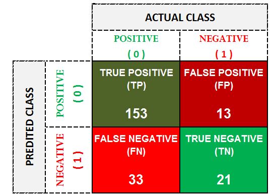
With the following confusion matrix, we know that the predicted number of defaulters is 166 (TP + FP) while the predicted number of non-defaulters is 54 (FN + TN). The total number of actual defaulters is 186 (TP + FN) while the actual non-defaulters are 34 (FP + TN). Now if we concentrate on the actual negatives, we can calculate specificity, which tells us out of the actual negatives, how many the model correctly predicted as negative, and from the above confusion matrix we get specificity to be at approximately 62% (TN ÷ (FP + TN) = 21 ÷ 34).

This means that as far as the defaulters are concerned, we are approximately 62% accurate in classifying the defaulters. However, many classification techniques such as Logistic Regression, Decision Trees and Naive Bayes don't explicitly provide us with class labels; rather they compute the probability of an observation belonging to a certain class. By default this threshold is set at 50%, which means that in our case any observation with a probability of more than 50% will be given the class label '1', i.e. labelled as a defaulter. As mentioned above, the various measures discussed under the confusion matrix can be easily manipulated, as a model predicting all observations as '1' will increase the Sensitivity, allowing us to classify all the defaulters correctly - however, by doing so we will end up labeling a lot of non-defaulters as defaulters, increasing the False Positives. This decision of how much False Negative or False Positive is admissible is very domain specific. For example, if Bank XYZ is liberal and can tolerate bad debts in order to grant loans to more people, the bank will want high Sensitivity and will tolerate low Specificity. However, if the bank is stringent and wants to be very cautious in dispersing loans, then it won't bother with low Sensitivity and will want high Specificity. All these measures depend on the values of True Positives, True Negatives, False Positives and False Negatives, which can be manipulated by altering the threshold value. For example, if we raise the threshold value to 90%, it will become tough for an observation to be categorised as 'Defaulter', and this will affect the various measures.

Thus we can say that the True Positive and False Positive Rates are simply a function of the threshold, and for different values of threshold we will have different values of such measures. This is where we take the help of the Receiver Operating Characteristic Curve, or ROC Curve, which is originally based on a military communication device used to communicate through radio and Morse code. With the help of the ROC Curve, we consider different threshold values and get to know the different values of True Positive Rate (Sensitivity) and False Positive Rate (1 − Specificity).

Sensitivity v/s 1 − Specificity

On one hand we have Sensitivity, which provides us with the percentage of positives that were classified correctly by the model, and naturally we want this number to be high. On the other hand we have Specificity, which indicates how good the model is at avoiding misclassification of the negatives, i.e. out of the actual negatives, how many the model correctly predicted as negative, and naturally we want this number to be as high as possible. If these values are high, it means that the diagonal values in the confusion matrix are high, indicating that the number of False Positive and False Negative observations is low. We want to see for which value of threshold these two numbers are highest; however, as we want both Sensitivity and Specificity to be as high as possible, it makes it difficult to plot their values on a graph for different values of threshold. Thus, rather than looking for very high Specificity, we look for a very low False Positive Rate, which indicates the percentage of negatives classified as positive by the model (basically the opposite of Specificity, i.e. 1 − Specificity).

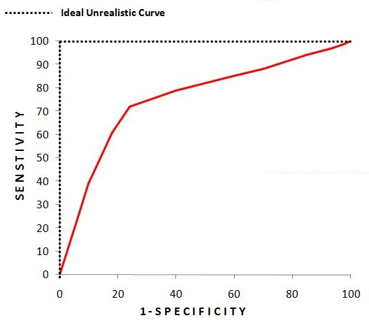
Now for different levels of threshold, when we plot the values of Sensitivity and 1 − Specificity, we get the following graph.

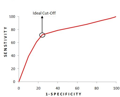
Here, for the Logistic Regression Model, we get different values of specificity and sensitivity for different values of the threshold. The ideal scenario would be a threshold that provides us with 100% sensitivity and 0% (1 − specificity); however, as this is generally not possible, we pick the next best thing, which is the ideal cut-off, where the difference between the two is highest, i.e. we pick the value of threshold where we have maximum sensitivity with minimum (1 − specificity). This is the point closest to the upper-left corner; the probability corresponding to it gives the best cut-off.

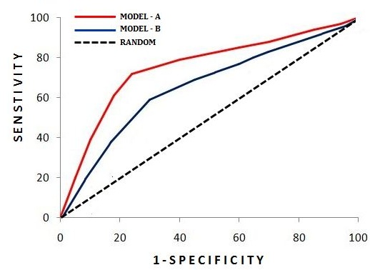
The ROC Curve can also be used to compare two models, as stand-alone values of different measures cannot make much sense on their own when comparing two models. Below we see, for different values of the threshold, the values of Sensitivity and 1 − Specificity for Model-A (Logistic Regression) and Model-B (Decision Trees). Here, no matter which threshold we consider for Model-A, it will provide better results than the results provided by the ideal cut-off of Model-B. The dotted black line represents the ROC curve of a completely random classifier. For example, if we have a dataset with an equal number of class label '0' and '1' observations, then a model that predicts all of them as 0 will produce this dotted line, as shown in the ROC curve.

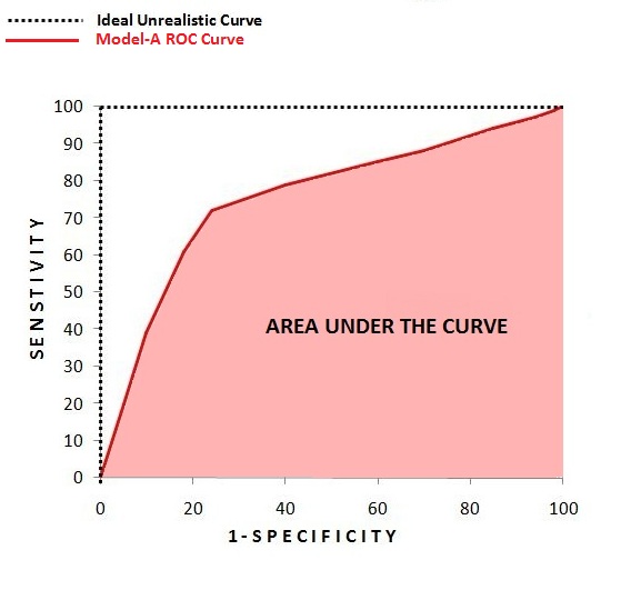
AUC Curve

It is a single-number metric that is an extension of the ROC Curve. Here we measure the area under the curve. For the perfect, unrealistic curve, the area under the curve will be 100%, while for a completely random model the area under the curve will be 50%. A model that performs worse than a random model will have an area below 50%. Here Model-A will be more accurate than Model-B, as the area under the curve is greater for Model-A than it is for Model-B. Thus the AUC Curve provides us with a single-value metric that quickly helps us understand the performance of the classification model.

If we compare a base rate model with a model that is more accurate, the difference between their AUC scores will be starker than the difference between their Sensitivity values.

Thus the AUC score provides us with a better idea of how the model is working, as with the ROC curve the difference between two models is sometimes not very visible, with the ROC curves of different models intersecting each other, performing better in some regions than others. The AUC score therefore provides us with a good overall evaluation.

Gini Coefficient

The Gini Coefficient tells us about the differentiating power of the model. In a ROC Curve, it is the area between the random model and the created model's ROC Curve.

The area between the random line and the model line tells us the additional lift that the model is able to achieve. The formula for the Gini Coefficient is 2 × AUC − 1.

Gain and Lift Charts

Unlike the Confusion Matrix and ROC/AUC Curve, Gain and Lift charts help us visualise the performance of our model in comparison to the base model/no model. Gain and Lift charts help us understand how our model is performing on different sections of the data. To understand how Gain and Lift charts work, let's take an example of a telecom company that wants to engage with its customers to reduce its attrition/churn rate, or in simple words, to stop customers from discontinuing service with the telecom company.

A prediction from a Base Model, or by having no model at all, provides us with a 10% attrition rate, i.e. on average, by the end of every year, 10% of the company's current customers discontinue the service. Thus if the telecom company has 100,000 customers, 10,000 of them will discontinue their subscription. However, the company has limited resources and cannot contact its entire customer base, and therefore requires some prioritization of customers so that it can divert its resources to those customers who are likely to churn.

We have the data of customers from the past year, and we build a logistic regression model to find the customers who eventually unsubscribed. Now, in addition to building a confusion matrix and ROC/AUC curve, we can also create a Gain and Lift Chart.

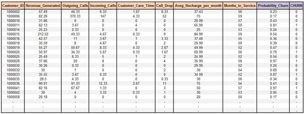
For every observation (details of a customer), the logistic regression model provides us with the probability of that observation being categorised as 1, 'Churn / Unsubscribed'. From the analysis of the ROC curve, we decide to go with a cut-off value of 0.7, which means that any observation with a churn probability of more than 70% will be declared as a customer who unsubscribed.

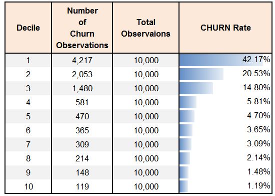
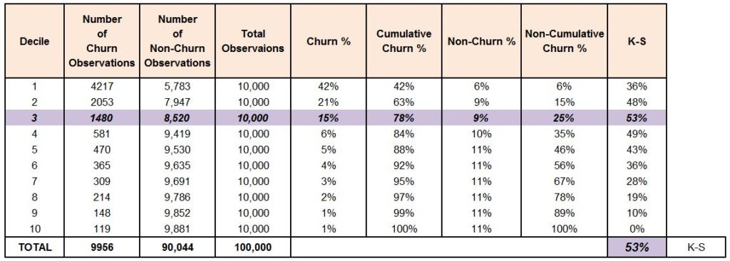
As Gain and Lift charts are based on the ordering of these probabilities, we sort the probabilities in decreasing order. We then perform deciling, or grouping, of the data - creating 10 deciles, each holding 10% of the data. We then calculate the number of churn observations captured in each decile and come up with the following table.

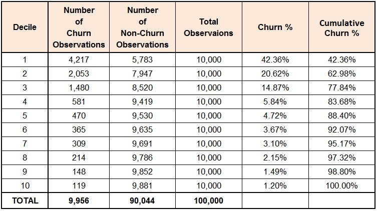
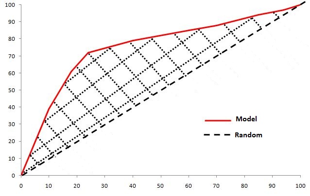
As per the table, we are able to capture almost 84% of the churners in the first four deciles. Before drawing any more inferences, we should create a gain chart, which is a line graph between cumulative churn % and cumulative population %.

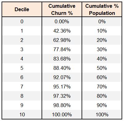
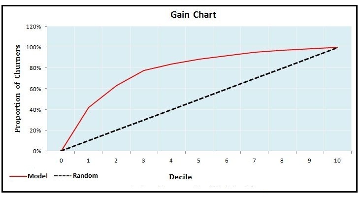
If we use a random model, each decile will have an equal number of churners, and the rate of capturing churners will increase by 10% perpetually for each decile. Thus, for the first decile, only 10% of all the churners will be captured, and similarly for the second decile we will capture another 10%, making the cumulative total 20%, and so on. The rate of capture is therefore equal to the percentage of observations in each decile. This would make prioritizing customers very difficult. However, when we use a model, we are able to capture 42% of churners in the first decile. The first decile only has 10% of the customers, yet from these 10% of customers, the model is able to capture 42% of the churners. A random model would have captured only 10% of the churners here. This 32% is the 'gain', or additional information, that the model has provided. Thus the rate of capturing churners is much higher when we use a model.

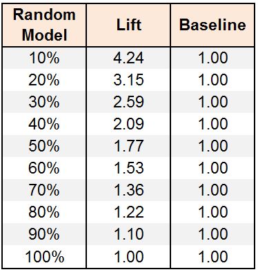
In the first decile, a random model would have captured 10% of the churners, while our model captures 42%. This means a lift of 4.24 times; therefore, by contacting only 10% of our customers, we are able to reach over 4 times the churn customers compared to a random model/no model.

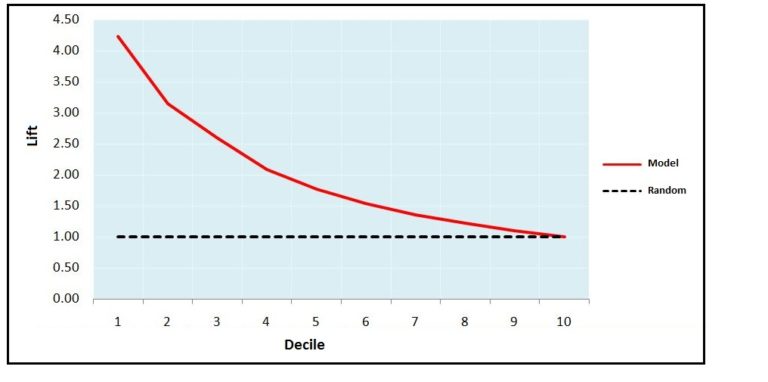
Lift charts help us target customers and plan campaigns by narrowing down our target population. However, our main aim here is to evaluate our model, and to do that we have to look for certain things that tell us how well the model is performing, such as: the lift generated in the first two deciles for a good model should be more than 2.0. In the gain chart, the area that falls between the random model line and the gain line can also be used as a measure to evaluate a model.

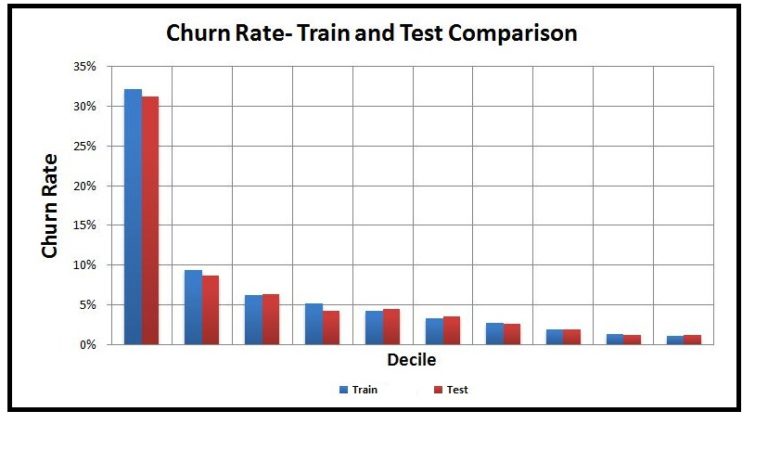
Also, the number of churn observations and the churn rate should perpetually fall with each decile (should follow rank ordering for at least 5 or 6 deciles). Here, churn rate for each decile is the number of churn observations divided by the number of observations in that decile.

Some validation can also be performed by making sure that the model, when run on the Train and Test datasets, has a similar percentage of churners (churn rate) in each decile, and it's better if the lines of both the models coincide with each other in the Gain and Lift chart.

KS Chart (Kolmogorov-Smirnov)

If we continue the above example, a Kolmogorov-Smirnov Chart will help us understand how good our model is at differentiating the customers who are going to discontinue (Churners) from the customers who are going to stay (Non-Churners). The KS statistic is the difference between the cumulative target and the cumulative non-target. In our example, as our target is churn, the KS statistic will be the difference between the Cumulative Churn and Cumulative Non-Churn observations. A higher KS value means that the model is good at separating the two classes. A KS statistic of 100 means that the model is able to create two mutually exclusive groups, each with a separate class label of observations. A KS statistic of 0 indicates a very poor model that fails to distinguish between the classes.

We can see that the maximum separation we receive is in the third decile. For a good model, the maximum KS statistic should fall within the top three or four deciles, as we expect the maximum differentiation between churners and non-churners to happen in the initial deciles only.

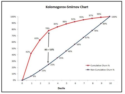
In our example, the KS statistic comes out to be 53%.

Concordance

It is one of the single most important metrics when evaluating a classification model's performance. To understand concordance, we can use an example where we have six observations, three having class label '1' (Defaulters) and three having class label '0' (Non-Defaulters). We then build a logistic regression model that provides us with the probability of observations belonging to class label '1'.

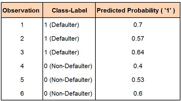
Our model will be concordant when, among all the pairs formed from '0' and '1' observations, the percentage of pairs is high where the probability assigned to the observation with class label '1' is greater than the probability assigned to the observation with class label '0'.

To put this in context, we first make all possible combinations of class labels '0' and '1' along with the predicted probabilities for them. In our example, we will form 9 such combinations/pairs.

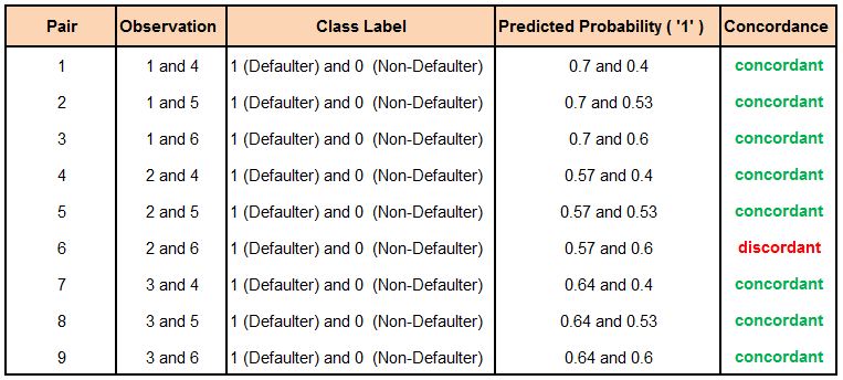
For the first pair, the probability of an actual defaulter defaulting is higher than the probability of an actual non-defaulter defaulting, meaning we have correctly categorised this observation. We similarly form 9 such pairs; however, in Pair 6, we get a discordant pair. Thus, out of the 9 pairs, 8 are concordant while 1 is discordant. Concordance is a ratio of such concordant and discordant pairs. In this example, the concordance comes out to be 88.9% ((8 ÷ 9) × 100).

In case the probabilities are the same (for example, 0.55 and 0.55), the pair is considered a tie and is neither concordant nor discordant.

Thus the model's segregation power matters for this metric, as concordance helps us understand how well the model segregates the negatives from the positives. The minimum accepted concordance for a model to be considered worthy is 60%.

All the metrics discussed so far play a crucial role in evaluating the performance of a model. We use these metrics during the training phase, and after evaluating a model's performance on the training dataset, we apply the model to the test set and again conduct a series of tests using the above-mentioned measures to evaluate the model. However, we need to validate a model in order to properly understand how well it performs with unseen or test data. To evaluate a model's performance with unseen data, we can perform various model validation methods, explored in the 'Model Validation' section.