// model evaluation

Regression Models

Various model evaluation techniques can be used under the supervised learning setup that help us in finding how good our model is performing. A very simple method to evaluate a model is by finding the accuracy, which is the difference between the predicted and actual values, however it is not a perfect method and can lead to poor decision making. Therefore we need other measures to evaluate the various models, and picking the right measure of evaluation is crucial in selecting and distinguishing the right model from other models.

In Regression, unlike classification (where we can count the number of observations that we have correctly classified) we are always wrong, as our predictions are either bigger or smaller than the original value (rarely is it the same as the original value). Thus we are not concerned with how many times we were wrong, but rather, with regression, what matters is the quantum of difference between the original and predicted values.

Sum Squared Error, Mean Square Error and Root Mean Square Error

It is the most common way of evaluating a regression model.

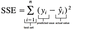
To find the Sum Squared Error, we first take the difference between the true and predicted value, we square it, and after summing them all up we get Sum Squared Error.

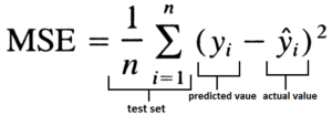
Sum Squared Error formula, the sum over the test set of the squared difference between actual and predicted value

If we divide this value by the number of observations then we get Mean Square Error.

Mean Square Error formula, one over n times the sum of squared differences between actual and predicted value

By taking a square root of MSE, we get the Root Mean Square Error.

We want the value of RMSE to be as low as possible, as the lower the RMSE value is, the better the model is with its predictions. A higher RMSE indicates that there are large deviations between the predicted and actual value. RMSE is a popular measure to evaluate regression models as it is easy to understand. RMSE functions on the assumption that the errors are unbiased and follow a normal distribution. RMSE is commonly used when selecting features, as RMSE is calculated with different combinations of features to see if a feature is significantly improving the model's prediction or not.

One drawback of MSE/RMSE is that it is sensitive to outliers, and thus outliers must be removed for MSE/RMSE to function properly.

Let's understand this with an example. We have a dataset with 10 observations and we apply two different models on them, and from both the models we get an MSE of 1. However, if we look in depth then we find that for the first dataset, the predictions had an error of $1 for all 10 observations, while for the second dataset, 9 out of 10 observations were predicted correctly while for the last observation the prediction of $4.16 was off by $3.16.

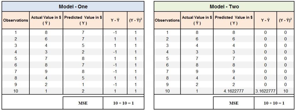
Two model tables, Model One with a uniform error of 1 across 10 observations and Model Two with a single large error of 10 from one observation, both producing an MSE of 1

Thus the drawback of MSE is that for it, a single big error will have the same effect as a lot of small errors, which happens because as we square the error in the formula, the single big error made by Model-Two has the same impact as the 10 small errors made by Model-One.

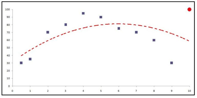
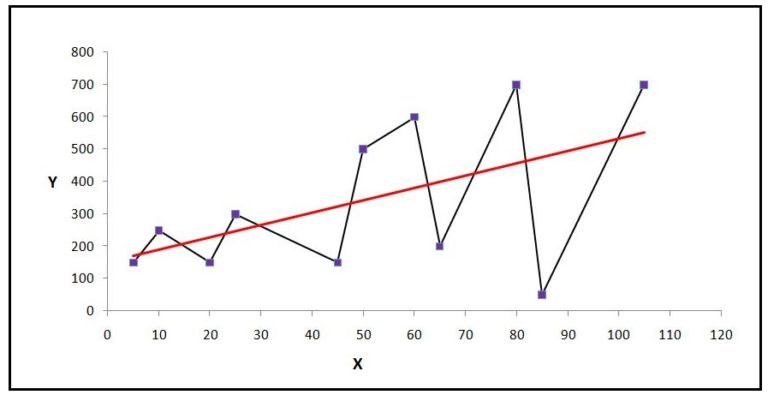
This problem becomes evident when we have outliers in our data. For example, a dataset with 11 observations where we have a dependent variable 'Stress Level' and an independent variable 'Results'. We fit a regression model on it and get a line of best fit and the following graph.

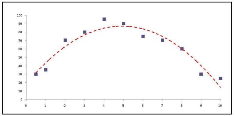
Scatterplot of Stress Level against Results with a curved line of best fit through the points

The points that form the line will be the predictions, and the distance from the actual data points to the predicted data point is the error. However, if we introduce an outlier, the model will try to accommodate the outlier, and in order to do so it will produce a different line of best fit, and this will cause the results to be skewed.

The same scatterplot with an added outlier point, causing the fitted curve to skew towards it and away from the other data points

Thus this happens especially when the metric used to calculate the error is MSE.

Another drawback of these measures is that, unlike Correlation Coefficients, they are sensitive to the mean and scale of predictions, i.e. if our model gets the correct mean, then it reduces the MSE significantly even when the pattern is completely missing. For example, in the above example, if our line of best fit is simply the mean of the actual values, then our MSE will be significantly lower than a line of best fit which gets the tendency right but misses the mean. Therefore for MSE, the baseline is the mean.

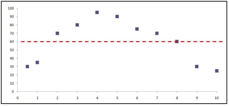
The same scatterplot with a flat horizontal line at the mean value used as the baseline prediction

Below, when the pattern is correct and the mean is wrong, the MSE will have a very low outcome, failing to provide us with the information that the pattern was predicted correctly.

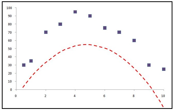
The same scatterplot with a correctly shaped but vertically shifted curve, illustrating a pattern-correct but mean-wrong fit

Thus the MSE is highly dependent and sensitive towards the mean and the scale.

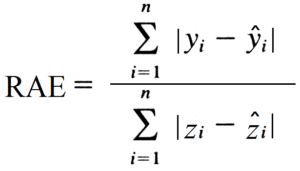
Relative Squared Error

It can be used to compare between models whose errors are measured in different units.

The formula for Relative Squared Error is

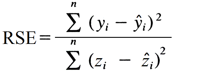
Relative Squared Error formula, the sum of squared differences between actual and predicted value divided by the sum of squared differences between actual value and a baseline mean predictor

We can use this method to solve one drawback of MSE, which is its sensitivity to the mean and scale of predictions. Here we divide the MSE of our model with the MSE of a model which uses the mean as the predictor, i.e. the line of best fit is simply the mean of the Y variable. This provides us with an output which is a ratio, where if the output is bigger than 1 then this indicates that the model created by us is not even as good as a model which simply predicts the mean as the prediction for each observation.

Mean Absolute Error

It is similar to MSE in the sense that here also we take the difference between the predicted and the actual value and divide it by the number of values, however instead of squaring this difference, we take an absolute value of it.

The formula for MAE is

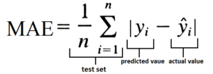
Mean Absolute Error formula, one over n times the sum of the absolute difference between actual and predicted value

If we don't take the absolute values, then upon summation the negative difference will cancel out the positive difference and we will be left with a zero. Therefore considering the absolute value of the difference is important. By taking the absolute values, MAE is able to deal with outliers better than MSE/RMSE. Therefore unlike MSE/RMSE, here a big error doesn't overpower a lot of small errors, and thus the output provides us with a relatively unbiased understanding of how the model is performing.

MAE is easy to understand, however it is not very popular, as it considers absolute values which undermine the reliability of this measure, and compared to MSE/RMSE it is less effective as it doesn't give higher weightage to large errors (which MSE/RMSE does by squaring the error terms). Unlike MSE, which has the mean as the baseline, MAE uses the median as the baseline, and if our model simply predicts the median then the MAE will be relatively smaller (similar to how a model predicting the mean will have a low MSE). Also like MSE/RMSE, MAE is very sensitive to the mean and scale of predictions. Thus MAE has its advantages and disadvantages, where on one hand it helps in dealing with outliers, but on the other hand, it fails to punish the bigger error terms.

Mean Absolute Deviation

It is similar to MAE with one crucial difference. In MAE, after taking the sum total of the absolute differences between the predicted and actual value, we divide it by the number of observations (i.e. we take an average of the differences between the predicted and actual values). In MAD we take the absolute differences between the predicted and actual values and then consider their median. By doing so, MAD becomes completely insensitive to outliers. However, the biggest problem with this metric is that we cannot take derivatives of it. As MAD is non-differentiable, it becomes difficult to update the betas in order to minimise the error. Thus unlike MAE, where we can take the derivatives, MAD doesn't provide us with this option, which makes this method quite unpopular. Also, it is similar to MSE/RMSE and MAE when it comes to being sensitive towards the mean and scale.

Relative Absolute Error

Like Relative Squared Error, it is also used to compare between models whose errors are measured in different units.

The formula for Relative Absolute Error is

Relative Absolute Error formula, the sum of absolute differences between actual and predicted value divided by the sum of absolute differences between actual value and a baseline mean predictor

Coefficient of Determination (R²)

Coefficient of Determination is the most important method of evaluating a regression model and is even more popular than SSE/MSE/RMSE. Coefficient of Determination (denoted by R² and pronounced as R-square) has been briefly discussed in the blog Correlation Coefficients. Following is an excerpt from Wikipedia about Coefficient of Determination.

In statistics, the coefficient of determination is the proportion of the variance in the dependent variable that is predictable from the independent variable(s).

It provides a measure of how well-observed outcomes are replicated by the model, based on the proportion of total variation of outcomes explained by the model.

The coefficient of determination ranges from 0 to 1. … simple linear regression where r² is used instead of R²

R² is a statistic that will give some information about the goodness of fit of a model. In regression, the R² coefficient of determination is a statistical measure of how well the regression line approximates the real data points. An R² of 1 indicates that the regression line perfectly fits the data.

In simple words, R² tells us how much variation in the dependent variable (Y) is explained by the independent variables (X).

SSR v/s SST v/s SSE

Mathematically, Coefficient of Determination can be found by simply squaring the correlation coefficient of the actual and predicted variable. However, to understand Coefficient of Determination, we should take a more visual approach.

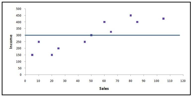
Now, for example, we have the following dataset with 'Sales' as the dependent and 'Income' as the independent variable.

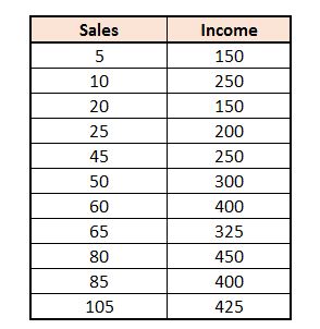
Table of Sales and Income data with 10 observations

We get the following graph when we plot the data points on a 2-D scatterplot.

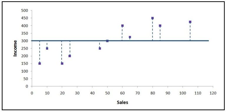
Scatterplot of Income against Sales for the 10 observations

SST

If we have a base model where, for every observation, the mean of the independent variable is considered as the predicted value, then we will have a line parallel to the x-axis.

The same scatterplot with a horizontal mean line drawn across the Income axis

An error here will be the distance from the 'blue average line' to the data point. If we calculate all such errors, i.e. consider the distance from each data point to the average line, square them, and then sum all these distances up, then we will get what is called SST (Sum of Squares Total). The value of SST is proportional to the variance of the data.

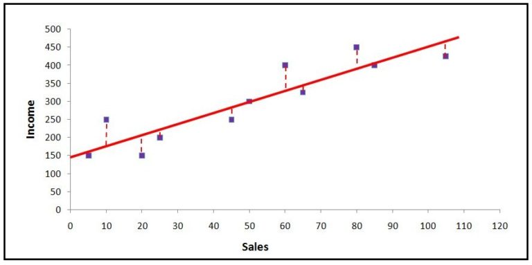
The same scatterplot with dashed vertical lines connecting each data point to the mean line, illustrating the SST error terms

SSE

Now we run a linear regression and come up with a line of best fit. We use the Ordinary Least Squares method, which means that the line considered best for prediction is that line which provides us with the minimum Sum Square Error (SSE), where SSE is the distance between the actual data points and the regression line. We calculate Sum of Square Error by calculating the distance between each data point and the regression line, squaring the distances, and then performing a summation. Thus this SSE, aka Residual Sum of Squares, tells us how much deviation there is between the actual and predicted.

The same scatterplot with a fitted regression line and dashed vertical lines connecting points to the line, illustrating the SSE error terms

SSR

Sum of Squares Regression (Sum of Squares due to Regression) is the distance between the average line and the regression line.

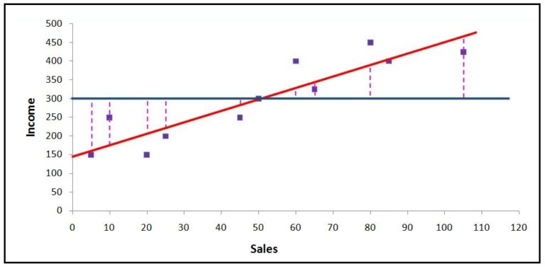
The same scatterplot with both the mean line and the regression line drawn, with dashed segments marking the gap between them at each x value

We can now use SST, SSR and SSE to understand how the variance is explained by each of them.

Let's consider the 9th observation (x=80, y=450). Here the distance between the average line and this data point is the total error (SST). SSR is the explained sum of squares, i.e. the error/deviation which we are able to explain. The distance between the regression line and this data point is the unexplained deviation. The total error is made up of explained error and unexplained error (SST = SSR + SSE). R² is a proportion of the total explained error/variation (R² = SSR ÷ SST).

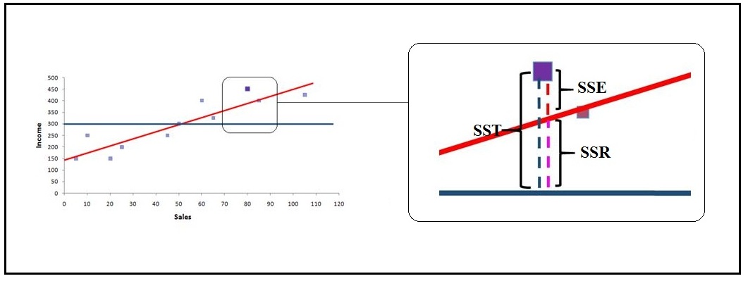
A zoomed-in view of the ninth observation showing the regression line, mean line, and the SST, SSR and SSE segments between them

Here, for the ease of explanation, we just considered only one observation, but for calculating R², we calculate the SSR (∑(ý−mean)²) and SSE (∑(y−ý)²) by considering all the observations. Thus Coefficient of Determination tells us how much variation/error can be explained - for example, if we have R² = 0.6 then what we can infer is that 60% of the changes that happen in the Y variable can be explained by the independent variables that we have used for creating the model. The rest 40% of the unexplained error can only be explained if we have more useful independent variables that can explain the variation in the dependent variable.

If we compare the Coefficient of Determination with the other metrics, then unlike MSE/RMSE/MAE/MAD, R² is not dependent on the mean and scale. However, there are two main enemies of correlation coefficients, and they are outliers and multicollinearity. As mentioned earlier, outliers cause the line of best fit to deviate in order to minimise the error in predicting their value. Multicollinearity, on the other hand, is a necessary evil. For example, for Linear Regression the assumption is that the dependent variable is correlated to the independent variables. However, if x1 is correlated to y and x2 is correlated to y, then there will also be a relationship between x1 and x2. When the relationship between the independent variables is too high, it causes multicollinearity, and it makes the model 'artificially good'. If the model has high multicollinearity, then this causes the R² to inflate, making the model unstable, as minor changes in a variable can change the output of R² drastically. Also, if variables are extremely related, then they don't explain any additional variance and become insignificant.

In least squares regression, R² increases with the number of regressors in the model. Because an increase in the number of regressors increases the value of R², R² alone cannot be used as a meaningful comparison of models with very different numbers of independent variables.

Thus we need a metric that can address the problem of overfitting, and this brings us to the next metric - Adjusted R².

Adjusted R²

Adjusted R² takes the number of variables into account when calculating the Coefficient of Determination, as it 'punishes' the extra variables being used in the model. To understand how Adjusted R² works, we first need to understand R² in terms of degrees of freedom.

As mentioned in the various blogs of Basic Statistics, degrees of freedom play a crucial role in calculating various inferential statistics, and its formula changes to a certain degree depending on the statistic we are calculating. In terms of R², we need to find degrees of freedom, as they provide us with the information on the minimum number of observations required in order to estimate a regression line.

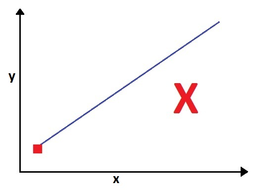
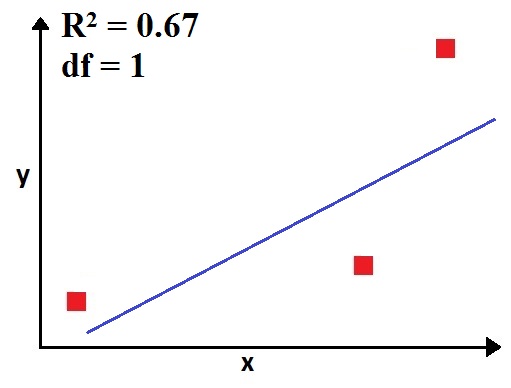
For example, we have a dataset with one dependent and one independent variable. We first start with our dataset having just one observation. If we plot the data on a graph, then it is evident that we can't have a regression line, as any regression line will start from the point.

A single data point on an x-y axis with no possible regression line, marked with a cross

Therefore, to have a regression line, we need at least two observations.

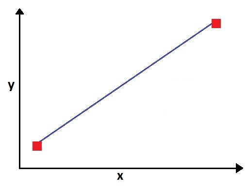
Two data points with a straight line drawn through them

Now we have a regression line, but it is meaningless, because no matter what the two points are, the R² will be 1, as the data points will always lie on the regression line.

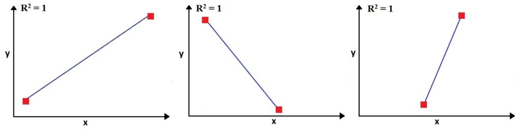
Three separate pairs of points each connected by a line, all with R-squared equal to 1 regardless of the line's slope or direction

It's only after the third observation that the model will gain some 'freedom' to assess the relationship between the x and y. Thus here the R² will change from 1, and the degree of freedom will be equal to 1.

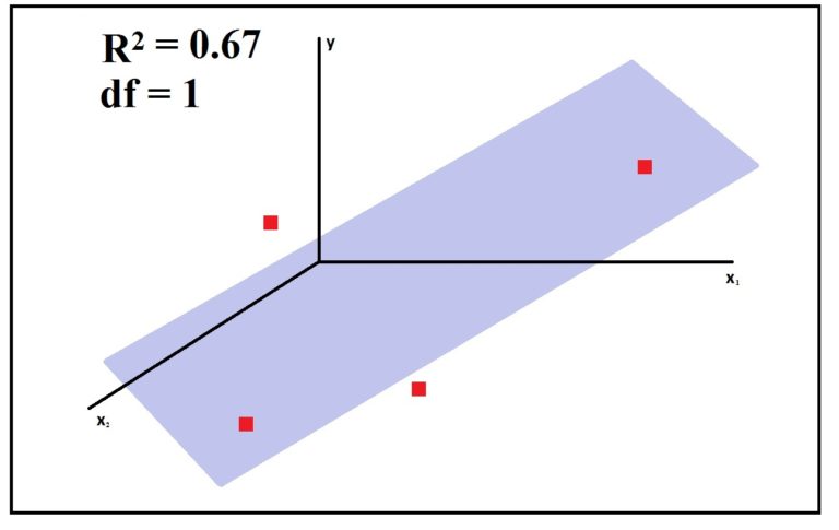
Three data points with a fitted line that does not pass through all of them, with R-squared 0.67 and degrees of freedom 1

The minimum number of observations that provide us with at least 1 degree of freedom depends upon the number of variables we are dealing with. For example, if we had two independent and one dependent variable, then we would have been dealing in a 3-dimension space. Here in multiple regression (when there is more than one independent variable), we won't have a regression line but a plane (plane of best fit). For the same three observations, now with an additional variable, the R² will be 1 and we will have no freedom.

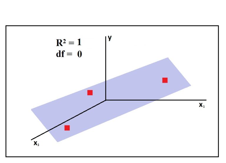
Three data points in a 3D space with a flat plane passing through all of them, with R-squared 1 and degrees of freedom 0

Thus any three data points in 3-dimensional space can have a plane that can cut all three of them, the way a line can pass through any two points in 2-dimensional space. Thus it is only after the fourth observation that we get a degree of freedom.

Four data points in a 3D space with a plane that does not pass through all of them, with R-squared 0.67 and degrees of freedom 1

Therefore df = N − K − 1

where,

df = degrees of freedom

N = number of observations

K = number of independent variables

Thus as the number of observations goes up, the degrees of freedom come down. (That is why it is required to have a large number of observations when there are a large number of features.) And in the above example, we found that an additional variable cost us one degree of freedom.

Now, how is all this related to R²? R² is affected by the degree of freedom because as the degree of freedom goes down (or in other words, more variables are added to the model), the line/plane/hyperplane of best fit becomes skewed and results in a high R². Therefore by including useless variables in the model, which don't explain any variance in Y, we can cause the model to overfit, as they will cause the degrees of freedom to go down, causing the R² to inflate. Thus R² can be deceiving.

The solution to this problem is Adjusted R². The formula for Adjusted R² is

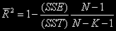
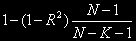
R-squared formula expressed as 1 minus the ratio of SSE to SST, each scaled by their respective degrees of freedom terms

Adjusted R-squared formula expressed as 1 minus the quantity 1 minus R-squared, scaled by N minus 1 over N minus K minus 1

The formula of Adjusted R² functions in such a way that as K increases, the values of Adjusted R² decrease, thus it keeps a check on the problem of multicollinearity. Generally, for a good model, the difference between its R² and Adjusted R² should not be much (the difference should generally be less than 0.05 - for example, if R² is 0.6 (60%) then the Adjusted R² should be between 0.55 and 0.6). Thus, Adjusted R² helps in accounting for the reduced power in the model due to low degrees of freedom.

Analysis of Residuals

Residuals are the differences between the actual values and the predicted values. If we square these errors and sum them up, then we get SSE (Residual Sum of Squares). A method to evaluate a model is by analyzing these error terms (residuals) by plotting them on a graph. Ideally, if the residuals appear to behave randomly and show no pattern, then it means that the model is good, however if it has some non-randomness to it, then it would mean that the model doesn't fit the data properly. Various types of visualization techniques, such as Scatter Plots, Run Charts, Histograms etc, can be used to analyze the residuals graphically. Also, a standardized residuals plot can also be used, where the errors are standardized, which when plotted, allows us to easily detect the outliers.