// classification problems

Logistic Regression

In this article, Logistic Regression will be explored. It is highly advised that you first go through Linear Regression, as the process and equation of logistic regression will be frequently compared with that of Linear Regression.

Logistic regression is used when the dependent variable is categorical. Unlike Linear Regression, where we have to predict a continuous value, in logistic regression we have to predict a categorical variable. Logistic Regression is a linear method of classifying the data, and it is not to be confused with Linear Regression, as a linear classification means classification is done by a linear separator (a line/hyperplane).

Logistic regression can be of three types: Binary (Binomial), Multinomial, and Ordinal. Binary Logistic Regression is when the dependent variable is dichotomous, i.e. it only has two categories; in Multinomial Logistic Regression the dependent variable has more than two unordered categories; and in Ordinal Logistic Regression the dependent variable has more than two ordered categories.

Each of these logistic regressions can either be simple, i.e. having a single independent variable, or can be multiple, where there is more than one independent variable. Binomial (Binary) Regression always codes the two categories in terms of 0 and 1.

In this article, simple Binomial logistic regression will be discussed.

Example Dataset

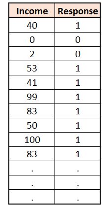
An example will help greatly in understanding logistic regression. Suppose we have a dataset where we have an independent variable ‘Income’ and a dependent variable ‘Response’. This dataset provides us information on the income of a person and the response of a credit card company when they applied for a credit card. The independent variable contains continuous (numerical) data, while the dependent variable is discrete, having two categories: 1 representing ‘request accepted’ and 0 meaning ‘request rejected’.

Just like we did in Linear Regression, here also we need to find that for a given value of x, what will be our y. Therefore we need to create a mathematical model that provides us with a probability of something happening or not happening for different values of x.

Difference from Linear Regression

The fundamentals of regression are the same, but still, linear regression cannot replace the need for logistic regression, as the fundamental difference is that the output of y is 0 and 1 and is not continuous.

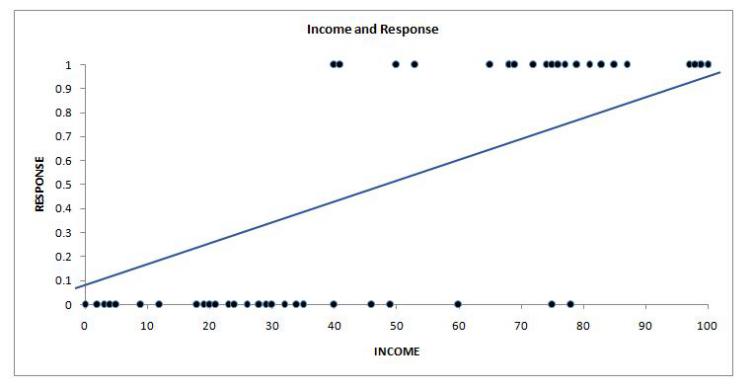
If we plot our dependent and independent variable on a scatter plot, then the best fit line will be of no good to us and won’t provide any meaningful result. This happens because the linear regression line is useful when both the dependent and independent variables are quantitative. Also, binary data (i.e. having only two categories) doesn’t have a normal distribution, which is a precondition for linear regression.

Also, distributions such as a U-shaped distribution can also be effectively used during logistic regression.

Also, unlike Linear Regression, Logistic Regression can handle data where the relationship between the dependent and independent variable is not linear, as logistic regression applies a non-linear log transformation to the predicted odds ratio (more on this ahead).

This is where logistic regression is used, as the model provides us with the probability of an event occurring depending on the values of the independent variable. These probabilities can be used in predicting the values of the dependent variable (based on a cutoff of the probabilities) and can be classified into binary numbers of 1 and 0. Like Linear Regression, Logistic Regression also helps in evaluating the effect of multiple independent variables on the dependent variable (in Multiple Logistic Regression).

Drawing parallels between Linear and Logistic Regression

As a linear function cannot be fit when the dependent variable is categorical, in such cases of a binomial distribution, a link function known as the logit function is used. The formula for the logit function is:

To start a rough comparison, we can say that the probability is calculated on the basis of the exponent of alpha and beta-x, which is divided by 1 + the exponent of alpha and beta-x. If you remember the equation for linear regression, which was Y = a + bx + e, then we can very roughly say that a + bx is a component that is present in the logit function, however we take an exponent of it. How we get to this function will be discussed below, but for now, let us stick with drawing parallels between linear and logistic regression.

The best fit line of linear regression represents the values if the dependent and independent variables are perfectly correlated. Thus all the data points that don’t fall on the line are considered an error term. If our data points lie on the regression line, then the scatterplot would look something like this:

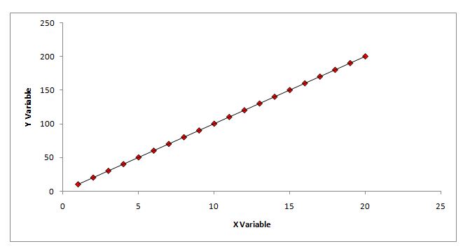
However, to proceed any further, it is important to understand the equivalent of this best fit line in terms of logistic regression.

For this, a simple example can be used. In a dataset, we have ‘years of education’ as the X variable and ‘employed’ (Yes/No) as the dependent variable (Y variable). We presume that the higher the years of education, the higher will be the chances of being employed. Thus as X increases, the probability of Y being 1 (Yes, i.e. employed) will increase. In our example we take a sample of 100 people, with 10 people having years of education ranging from 0-2, another 10 having years of education from 3-4, and so on. Then we take the average number of employed people (1) in each group, i.e. we compute the mean score on the dependent variable for each category of the independent variable. This mean is nothing but the probability of finding 1. This is also the reason that the inverse logit function (which will be discussed ahead) is known as the mean function. The perfect scenario will be what has been mentioned above, where for an increase in the number of years of education, the probability of having 1 (being employed) increases.

Such data and a graph will look something like this:

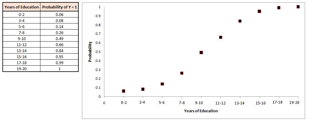
If you look closely, you can see how the data points are different from a regression line. Here the data points take an S-shaped curve, also known as the sigmoid curve, which happens when we plot the average values of y for different values of x. These average values can also be said to be the expected values, or the desired values. And this desired curve is formed when, for an increase in x, the probability of y=1 increases.

A perfect S-curve means that a perfect relationship exists between the independent and dependent variable, and here in logistic regression we hope for an S-shaped line rather than a simple straight line, which we find while performing linear regression.

This S-shaped line has a function the way the best fit line in linear regression had, and this function is known as the logit function.

There are many other parallels that can be drawn between logistic and linear regression, and they will be mentioned while exploring the logit function.

Logit function

For understanding the logit function, we have to understand 5 equations one by one that will help us in drawing inferences from the output. These 5 equations are:

1) odds = P ÷ (1−P)

2) odds ratio = (P1 ÷ (1 − P1)) ÷ (P0 ÷ (1 − P0))

3) logit(P) = ln(P ÷ (1−P)) = (a + bx)

4) Inverse Logit / Mean function = logit^-1(a) = 1 ÷ (1 + e^-z) = e^z ÷ (1 + e^z)

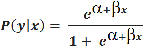
5) Estimated Regression Equation = p̂ = e^z ÷ (1 + e^z) (where z = a + bx) = e^logit(P) ÷ (1 + e^logit(P)) = e^α+βx ÷ (1 + e^α+βx)

Odds

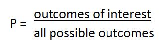
To understand odds, we first review probability. Here P is equal to the outcomes of interest divided by all possible outcomes.

For example, if we flip a coin, then P = 1 ÷ 2; this means that the probability of heads will be 50%. Similarly, if we roll a die, the probability of finding a 1 or 2 will be 33% (2 ÷ 6 = 1 ÷ 3 = 0.333).

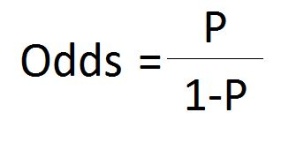
The odds are the probability of an event occurring divided by the probability of that event not occurring. It can also be said to be the probability of scenario A occurring divided by 1 minus the probability of scenario A occurring. Therefore the formula for odds is P ÷ (1−P), where P means the probability of a particular event occurring.

You must remember that here the probability value cannot be more than 1. Coming back to our example, the odds of having heads after flipping a coin will be 1 (we can also say that the odds of getting heads are 1:1). This can be calculated by using the above-mentioned formula: 0.5 ÷ (1 − 0.5) = 0.5 ÷ 0.5 = 1.

Similarly, the odds of getting 1 or 2 after a die roll are 1:2, i.e. 2 ÷ (6−2) (i.e. 0.333 ÷ (1 − 0.333)) = 2 ÷ 4 (i.e. 0.333 ÷ 0.666) = 1 ÷ 2 (i.e. 0.5), i.e. 1:2.

But why do we need to understand odds? We need to understand odds so that we can understand odds ratio.

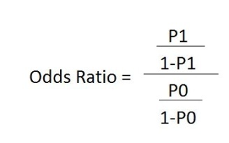
Odds Ratio

As the name suggests, the odds ratio is the ratio of two odds. The formula for the odds ratio is:

To understand this, let’s take an example where we have a loaded coin where the probability of having heads is higher than that of finding tails. Here, for example, the probability of finding heads is 0.7. Thus if we compare this coin with our normal coin, we can find the ‘odds of having heads in the loaded coin’.

Therefore here our equation will be:

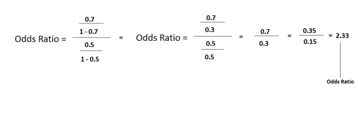
Thus the odds of getting heads with a loaded coin compared to a normal fair coin is 2.33 to 1, i.e. the odds of getting heads is 2.33 times greater than the chance of getting heads with the normal coin.

Why do we need to understand odds ratio? We need to understand odds ratio because, in logistic regression, the odds ratio explains how much increase/decrease will happen in the probability of finding an outcome (of the Y variable, for example finding the outcome being 1) for a unit increase in an X variable, holding all other independent variables constant. For example, if we have a dependent variable diabetes and an independent variable weight, and if the odds ratio of the independent variable comes out to be 1.09, then this will mean that a kilogram of increase in weight will increase the chances of having diabetes by a factor of 1.09, which will be 9%. So if this odds ratio had been 2, then it would have meant that a unit increase in weight will increase the probability of having diabetes by a factor of 2, which will be 100%. This information plays an important role in evaluating the importance of independent variables and their effect on the dependent variable’s probabilities.

Then does it mean that the odds ratios are the coefficients of Logistic Regression, as it provides the same information that the coefficients of linear regression provided (how much increase in Y to expect for a unit increase in X)? Well, the answer is not that simple. In logistic regression, we do get the regression coefficient (b) for every independent variable; however, because of the complicated algebraic translations, these coefficients cannot be interpreted the way we did in linear regression. So if we have a dataset having an independent variable ‘Income’ and a dependent variable ‘Response’, where we are trying to find probabilities of the response being ‘1’, and we get a coefficient of 0.013529, then this will not mean that a unit increase in income will increase the chance of the response being 1 by 0.013529 times (1.3%). However, the knowledge of odds ratio will come in useful, as the exponent of this coefficient (exp(b) or e^b) is the odds ratio of the independent variable. Thus if we take the exponent of the regression slope, which in our example is 0.013529, then the odds ratio will be 1.0136. This means that it is 1.0136 times as likely to get Y=1 for every unit increase in the X variable. For example, if our coefficient value had been 0.70128, then the odds ratio would have been 2.016332, which would have meant that the dependent variable being equal to 1 is twice as likely for a unit increase in the X variable (2.01 times). However, if the coefficient value was zero or very close to 0, then it would have meant that there is no relationship between the independent and dependent variable (the odds ratio then would have been 1), while if the beta value was, for example, negative, having a value of −0.691789, then the odds ratio would have been 0.5068, meaning that for a unit increase in X, the probability of getting y=1 is half as likely, meaning there is a negative relationship between the two variables.

Do high Odds Ratio and Probability mean the same thing?

It can be easy to confuse probability and odds ratio; however, there is a subtle difference.

Let’s use the ‘Income’ and ‘Response’ dataset, where Response is the dependent variable, with y=1 meaning ‘request for the application of credit card accepted’. We input this dataset into the statistical software, and in a logistic regression model, where we come up with the a and b values, and by using them as inputs in the logit function (to be discussed below), it is able to provide probabilities of Y=1 for different income values (the independent/x variable).

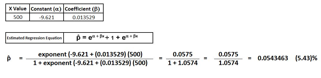
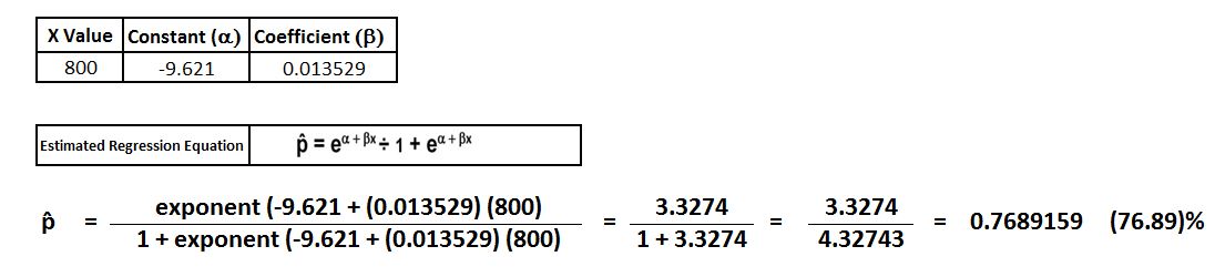
Let’s say in the output we find that the constant (a) is −9.621 while the coefficient (b) is 0.013529. We know that here the odds ratio will be 1.013621, meaning that a unit increase in income will increase the chance of the response being 1 by a factor of 1.013621 times. Now we can use the logit function to find the probability for various values of income, and for a second let’s get a bit ahead of ourselves and input these values into the Estimated Regression Equation, which is p̂ = e^α+βx ÷ (1 + e^α+βx).

For an x value of 500, the probability of Y=1 comes out to be 0.0543463 (5.43%).

If we increase the x value by 300 (to 800), the probability of Y=1 comes out to 0.7689159 (76.89%).

This shows that for this increase of 300 in the value of x, the probability of Y=1 increases by 71.46%. If we have to calculate the odds ratio, then we can use the odds ratio formula and input the two probabilities to find the odds ratio for these two values of X.

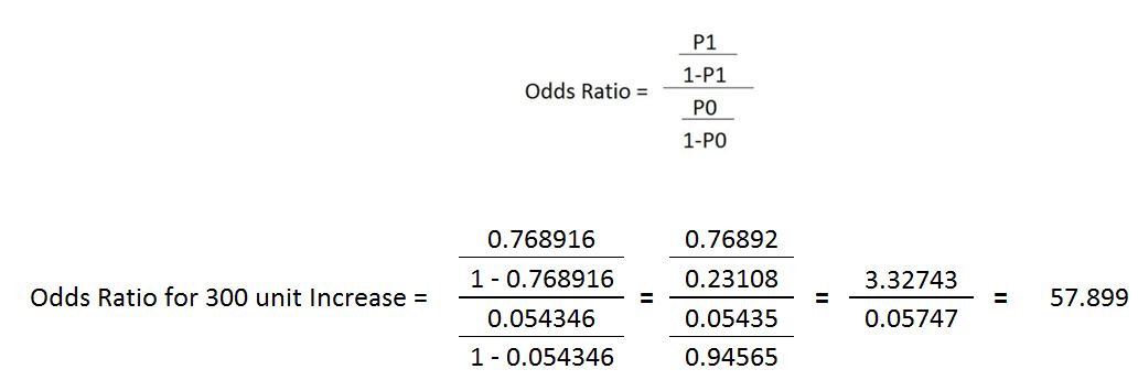
Thus it is 57.899 times more likely to get Y=1 for a 300-unit increase in the X variable.

However, it is important to understand that probability and odds ratio are two different things. The probability of being accepted for people with less income will be lower, while the probability of being accepted for people with greater income will be high. On the other hand, for every increase of 300 units in income, the odds of being accepted will increase by 57 times (57.899), and this holds true at any point in the income spectrum/range. So if the income increases from 801 to 1101, then the odds of getting Y=1 will remain constant, at a factor of 57.899, i.e. 57 times, however the probabilities of Y=1 will fluctuate.

We can do some calculation to understand this.

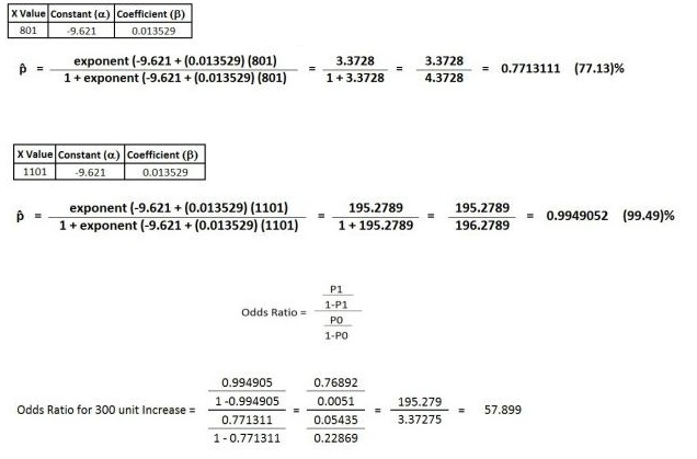
We can see above how an increase of another 300 units of X increased the probability of having Y=1, but this time the probability increases by 22.36% rather than 71.46%, as it did when the value of x increased from 500 to 800. Thus the higher the income, the higher the probability here. However, the odds ratio remained the same (57.899). Therefore the odds ratio is the same for any equal interval in an independent variable; thus a person increasing income by 300 increases the odds of being accepted by a factor of 57.899 regardless of their starting income. However, the probability of being accepted is already very low for people with less income to begin with. So while the odds are 57 times greater, the starting probability will still be low if the income is less. So a large magnitude of odds can be there even when the probabilities are low.

To understand this intuitively, the probability of finding a movie star on your way home and finding an alien at your doorstep are both very low, but the probability of finding a movie star is very high when compared to the probability of finding an alien, making the odds of finding a movie star much higher even when the underlying probability of it happening is very low.

If we have to find the odds ratio through coefficients only, then what is the method to calculate the coefficients? Unlike Linear Regression, where the coefficient could be found using a method known as Ordinary Least Squares, where the line of best fit was constructed by minimizing the squared residuals (or simply the difference between actual and predicted data points), in Logistic Regression the constant and coefficient value is calculated using a method known as Maximum Likelihood Estimation (MLE). MLE uses a very different algorithm to find the alpha and beta. MLE is used rather than the old, simple OLS because here we don’t predict values of Y but predict probabilities of a dichotomous variable, and because of this, OLS cannot be used, which requires a presumption of the residuals being normally distributed. Thus we make an algebraic conversion of the linear regression equation and use MLE for finding the constant and coefficient. However, getting into the details of how the coefficient and constant value are calculated using MLE is beyond the scope of this article, and it is highly recommended that you do your own research on this. Still, to give you some idea, Maximum Likelihood tries to find the smallest deviance between the observed and predicted values, and tries to find something like the best fit line of linear regression, with statistical software performing multiple iterations in the backend until the minimum variance is found (also, as it tries to find the difference between observed and expected, it is something along the lines of chi-square, and is the reason that when using software for performing logistic regression, terms such as chi-square and Wald chi-square can be found in the output).

Logit Equation

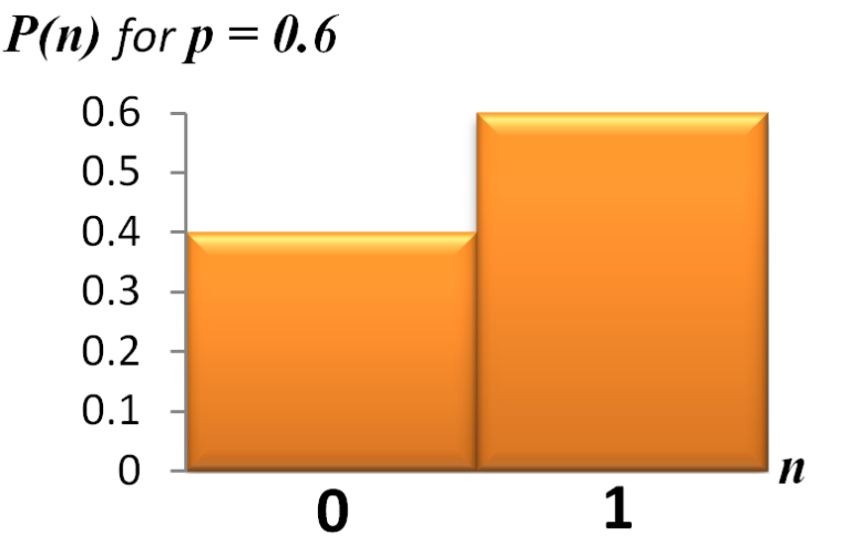
The dependent variable here doesn’t follow a Gaussian distribution (explained in Measures of Shape, where it was discussed that there can be multiple probability distributions) but follows a Bernoulli distribution having unknown probability (P). To simply explain what a Bernoulli distribution is: it is simply the probability distribution of any single experiment that has a binary outcome (0 or 1, yes/no, etc.). For example, if we flip a coin just once (we want heads to be the result), then such data will have a Bernoulli distribution, having a probability of having heads as P and tails as 1−P. The random variable that represents the trial is known as a Bernoulli random variable.

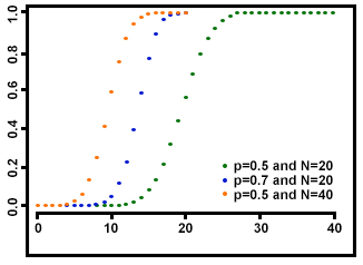
However, if we flip the coin 5 times (i.e. conduct n number of independent experiments) with each experiment/trial having its own probability, then each of these flips of the coin will be a Bernoulli trial, and their sum will form a binomial distribution with parameters n and p. Thus a Bernoulli distribution is just a special case of a Binomial distribution where n=1 (that is, just one trial), while a Binomial distribution is made up of multiple independent random variables, each of them being Bernoulli distributed with success probability P. (For a single trial, binomial distribution = Bernoulli distribution.)

In logistic regression, we have to estimate this unknown probability for any given combination of the independent variable. So in our example, for a value of x, a logistic model can be used to find the probability of Y=1. Thus there is a need to link the dependent variable having probabilities (a Bernoulli distribution) with the independent variable having various values, and this link is known as the logit link.

As in logistic regression we have to find the P, the goal becomes to estimate the P (p̂) for a linear combination of independent variables. To tie together the linear combination of variables with the Bernoulli distribution, we need the logit function that helps in linking them together. Thus it maps the linear combination of variables that could result in any value onto the Bernoulli probability distribution (ranging from 0 to 1).

This logistic (logit) function is simply the log (natural logarithm) of odds, i.e. ln(P ÷ (1−P)). This natural logarithm of odds is the logit of probability.

Also, the natural log of the odds (ln(P ÷ (1−P))) is equal to the linear function, i.e. the linear combination of the independent variable, which is α + βx (the linear regression equation).

Thus by using this function we get a sigmoid curve, and the following log link function graph can be drawn:

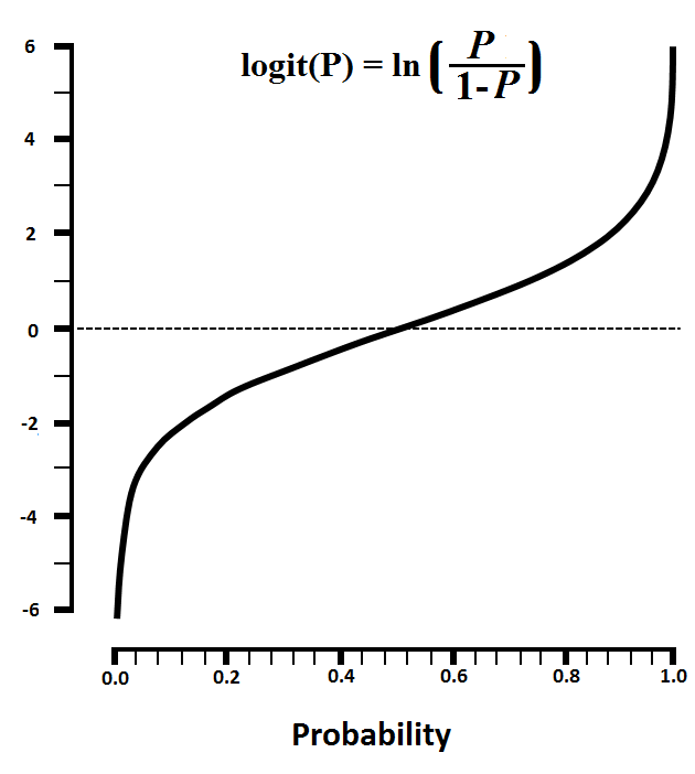
Here the probabilities run on the X-axis and range from 0 to 1, and a curve is formed on the basis of Maximum Likelihood Estimation, through which we will predict the probabilities for different values of x.

Inverse Logit / Mean function

Inverse Logit, or the inverse log odds, is used as we need the dependent variable, which here is the probability, to be on the Y-axis (refer to Linear Regression, where the dependent variable was always on the Y-axis when finding the Best Fit Line). Thus to make the probabilities run on the Y-axis and have a sigmoid (S-shaped) function curve, the inverse logit is used. When we use the inverse logit, it provides us with probabilities of Y=1 for values of x.

logit^-1(a) = 1 ÷ (1 + e^-z)

In the above formula, the inverse logit is found by taking the exponent of something (z). Remember that the exponential function here, symbolised by ‘e’, is the opposite of the natural logarithm (ln). Also, do not confuse the exponential function symbol ‘e’ with the ‘e’ found in the linear regression equation, as there the ‘e’ meant residual/error, while when the symbol ‘e’ is used to refer to the exponential function, the symbol always has a superscripted value attached to it.

The above formula can also be written as e^z ÷ (1 + e^z).

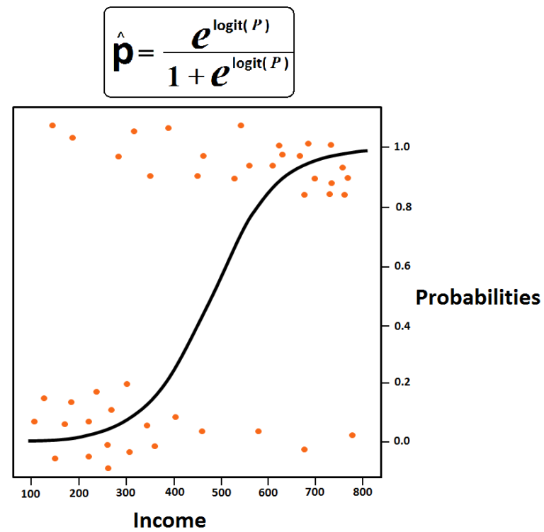
Estimated Regression Equation

The estimated regression equation provides us with the estimated probabilities (p̂). This equation is found when we use the inverse logit function and express the something (z) as α + βx. Thus by doing so we simply take the antilog, i.e. the exponent of the logit function.

The equation can be expressed in the following ways:

p̂ = e^z ÷ (1 + e^z) (where z = α + βx)

p̂ = e^logit(P) ÷ (1 + e^logit(P))

p̂ = e^α+βx ÷ (1 + e^α+βx)

Thus the above equations make the probabilities run on the Y-axis, providing a sigmoid (S-shaped) function curve to predict probabilities of Y=1.

Multiple Logistic Regression

When there are multiple independent variables, the equation has multiple coefficients (just like it did in linear regression) and becomes something like:

e^{α+β1x1+β2x2…+βnxn} ÷ (1 + e^{α+β1x1+β2x2…+βnxn})

With multiple logistic regression, we don’t get a curve but get a wave, as we are dealing with a 3-dimensional space (i.e. when having two independent variables). Such a graph looks something like this:

Thus logistic regression can be used when the dependent variable is dichotomous. Here the linear regression equation is transformed into an algebraic equation, and probabilities are used to find if Y will be 1 or 0; however, this depends on the cutoff of the probability, as the standard cutoff is at 50%, therefore any linear combination that provides a probability of more than 0.5 is termed Y=1, and lower than 0.5 is considered Y=0. This cutoff value has to be tweaked. Also, the methods of evaluating a logistic regression are very different from linear regression, as we don’t have an R². All such aspects related to evaluating the model have been explored in Model Evaluation & Validation for Classification Models. Since we are working here with a binomial distribution (dependent variable), we need to choose a link function that is best suited for this distribution, and it is the logit function. In the equations above, the parameters are chosen to maximize the likelihood of observing the sample values, rather than minimizing the sum of squared errors (as in ordinary regression). Logistic Regression is the most common algorithm used for classification problems and can provide good results even when compared to much more sophisticated methods such as SVM and ANN.