// classification problems

Artificial Neural Networks

Neural Networks is one of the most advanced methods to solve Regression and Classification problems. The working of Neural Networks is inspired by the human brain, which consists of billions of neurons.

Evolution of Artificial Neural Networks

Phase 1

Artificial Neural Networks were first used in the 1940s, when Warren McCulloch and Walter Pitts, in their paper ‘A Logical Calculus of Ideas Immanent in Nervous Activity’ (1943), built models which worked the way human brains did. These early models were based on the working of a single neuron that had a binary threshold activation function. These models were a good stepping stone; however, such models could only solve simple problems and weren’t of much use. The development of artificial neural networks was put into cold storage after a book named ‘Perceptrons: An Introduction to Computational Geometry’, written by Marvin Minsky and co-authored by Seymour Papert, was published in 1969, where they proved the weaknesses and showed how the neural networks present at that time could only solve linearly separable functions and couldn’t solve simple boolean problems such as XOR and NXOR functions. Marvin Minsky and Seymour Papert even stated that research on the perceptron was doomed to failure.

Phase 2

However, research kick-started in the 1980s with the discovery of two things: first was the knowledge to put multiple perceptrons together, and the second was Backward Propagation. But the knowledge of applying Neural Networks successfully was held by very limited people and couldn’t be used universally. Also, the technique was very computationally expensive, and the computers available at the time couldn’t handle it. Meanwhile, the development of other successful linear techniques such as Support Vector Machines, developed by Vladimir Vapnik and Alexey Chervonenkis, caused an end to the progress of Neural Networks.

Phase 3 (Present)

Neural Networks were reborn in 2013-14, mainly due to a revolution in computer hardware resulting in an exponential increase in processing speed, which made the use of heavily computationally intensive neural networks viable.

Why Neural Networks Stand Out

The basic equation of all machine learning algorithms (for example, a classification problem) can be written as Y = sign(wx + b). Here Y is the predicted value while x represents the input data. We are then left with w, which is the weight, and we have to find whether it is more than 0 or less than 0. With regression, the sign is removed and we are left to find the value of the weight which will impact the predicted value. However, these weights heavily rely on the right set of features, and it becomes difficult in the case of a different kind of data, such as data pertaining to multimedia, which has a very different kind of feature set from the features discussed so far.

For example, if we have an audio tape, then it cannot be used as an x variable, as the model won’t learn anything. Thus we transform x, and for that we need a lot of domain knowledge. For example, if we have ten images, then we can’t just take their pixel intensities as data and use them as x variables, as we don’t know which of those features represent the curvature, edges, colors, basic shape, etc. For this, we would be required to apply edge detectors, for which in-depth domain knowledge would be required.

Thus we require a universal learning algorithm that can understand all kinds of data, no matter whether the source of it is an image or audio. At this point, it becomes interesting to ask a question: how are kids, who don’t have ‘in-depth domain knowledge’ about the geometry of fruits, able to distinguish one fruit from another? The answer lies in our brain, which is able to convert all the data into features that can be represented in a way understood by a universal learning algorithm, and that algorithm is a neuron.

The process of training such a learning algorithm is similar to teaching a kid to recognize different fruits, where we start by telling them what is what, and once told, we keep on asking them about it and keep on correcting them until they are able to recognize patterns which lead to better results.

Parallels between Neurons and Artificial Neuron

Working of Neuron

To understand how an Artificial Neuron works, it is important to first understand how a Neuron functions and draw parallels between them.

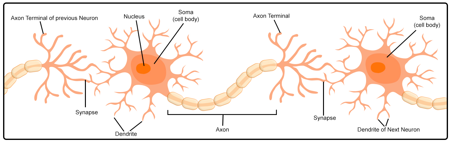
Humans don’t need feature representation, as we have cells in our brains known as neurons. Each neuron has a body wherein the middle lies a nucleus. The body of the cell (Soma) has tentacle-like structures sticking out in different directions, which are known as dendrites. From the Soma, one of these dendrites is elongated in a direction and is known as the axon. For our understanding of artificial neural networks, we only need to understand the working of these parts of a neuron.

The dendrites are sensitive to certain kinds of chemicals, and when they absorb the chemicals, they generate a chemical signal which is transferred to the nucleus. If the amount of chemical is more, then it causes the dendrites to produce a stronger signal, and if the strength of the signal is beyond a certain threshold, then it causes the nucleus to fire an electrical pulse. This electrical pulse is then sent through the axons down to the axon terminal. When it reaches the axon terminal, the signal causes another chemical reaction. The axon tips release the chemicals in the synapse, which is the gap between the two neurons. This chemical is then picked up by the dendrites of the other neuron.

The whole process is then repeated, and if the signal strength is able to overwhelm the nucleus of this neuron, then it fires, which is then picked up by another neuron and so on; however, if it doesn’t produce a strong enough signal, then the other neuron doesn’t fire. Thus here the amount of chemical and the threshold after which the nucleus fires play a major role in producing the electric signals, and a human brain produces enough of such electric signals to generate enough electricity to light up a 25-watt bulb.

Artificial Neuron and parallels between Neurons and Artificial Neuron

With the understanding of the working of a neuron, we can create a mathematical model. This mathematical model, based on human neurons, is what gives rise to the artificial neural network.

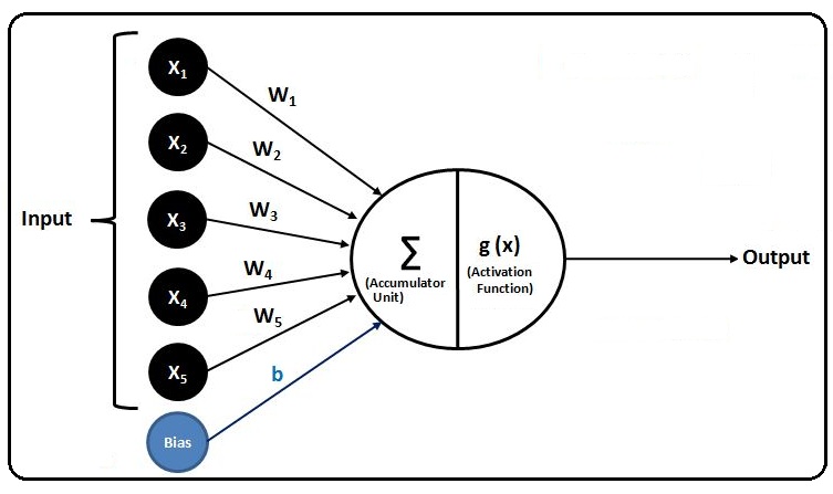
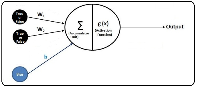
For example, we have a classification problem at hand, and we have five ‘x’ variables which will be our input variables. The value of the x variables is then fed into an ‘accumulator unit’. The accumulator unit adds the values of these input variables to find out how much ‘chemical’ is there. Thus it simply does the summation and comes up with a value.

Till now we have replicated the chemicals and the dendrites, but now we need something parallel to the nucleus found in the neuron. To replicate the firing mechanism of the nucleus, we use something known as an activation function. There are a lot of activation functions. For now, as an example, we consider a squashing function (sigmoid) which squashes the activation between 0 and 1, and we use a threshold value. So if the value is less than the threshold, then it fires 0, and if it is more than the set threshold value, then it fires 1.

The activation unit, if modeled on a sigmoid, will have an equation g(z) = 1 / (1 + exp(−z)), where z is the value provided by the accumulator unit. Thus the activation function generates a value of Y which is a function of the x variables, weights, and bias. The Y here can be understood as the electrical signal produced by the nucleus.

We also use weights as input in the accumulator unit. The idea behind using weights can be understood from dendrites having different strengths to pick up the chemicals (x variables). Therefore, if the strength of a dendrite is high, then it produces a high signal, and vice versa for the same value of an x variable. This strength of dendrites is manifested through the use of weights, where the input variables are assigned weights, and the values of these input variables are then multiplied by their respective weights to mimic the effect of the different strengths of dendrites.

Till now we have picked up the chemicals (input x variables), multiplied them by the strength of the dendrites (weights), and added them all up using an accumulator unit. However, we also add a bias term. In a binary classification problem, a bias can be easily understood as a value which acts as a boundary for the value of input which it requires to cross in order to jump from one class to another.

Now all this information is sent to the activation function, which determines the behaviour of firing. With this, we come up with the final equation for an artificial neuron, which is:

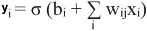
Interestingly, we had input variables, a squashing function (sigmoid), and output Y, which is a squashed version of a weighted sum of inputs. This is the same as Logistic Regression. Thus, so far, we have been able to achieve what logistic regression can also do.

Limitation of Artificial Neuron

So far we have created a model known as a Single Layer Perceptron, where we use only a single neuron. Remember, this is where it all started in the 1940s. To understand the limitation of a single-layer neuron, we will explore and try to solve a simple boolean problem which cannot be solved by a single neuron, as pointed out by Marvin Minsky and Seymour Papert in their book ‘Perceptrons’. This boolean problem is known as XOR.

The basic understanding that we get from their book is that a single neuron can only solve linearly solvable problems, and for example, if we have data for 28-pixel images having handwritten digits from 0 to 9, which will provide us with 784 features (28 × 28 = 784), and we use these 784 features to classify the 10 digits, and if these data points are not linearly separable in any dimension, then the single neuron will not be able to help us in any way.

In real life, a lot of problems cannot be solved through linear separators, and to demonstrate this we will work through the XOR problem.

If we have to create a ‘Truth Table’ using the boolean operator ‘and’ (&&), then we should know that True and True = True, True and False = False, False and True is False, while False and False = False.

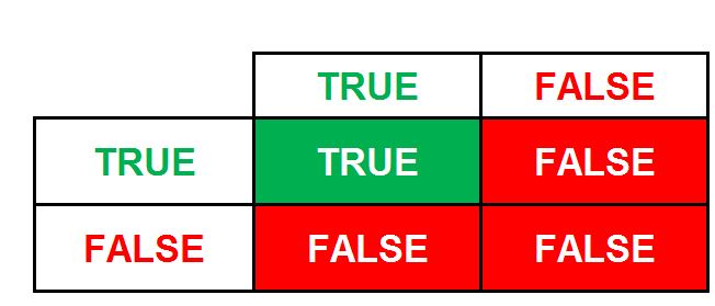
Now if we have a boolean expression ‘A && B’, and in order to get True, we require both expressions A and B to be true. Interestingly this is a linearly separable problem, as all the False values can be on one side and True can be on another (i.e. if A is true and B is true, then only True; for example, A is Age=25 and B is Balance=50; then if Age is not 25 and Balance is 50, then false; Age is 25 but balance is not 50, then false; both Age and Balance not being 25 and 50, then false).

Thus if we have to create a single-layer perceptron, then we can do it by having two input variables, True and False. We can then train this model where when two Trues come in we will have a True, while for the others we will have False (True False, False True, False False).

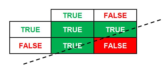
If we change our boolean expression to ‘A || B’, i.e. if in place of having the boolean operator ‘and’ (&&) we have ‘or’ (||), the truth table changes; however, it will still be linearly separable, meaning that we can still use a single neuron to solve this problem.

(i.e. if either A or B is true, then True; for example, A is Age=25 and B is Balance=50; then if Age is not 25 and Balance is 50, then true; Age is 25 but balance is not 50, then true; both Age and Balance being 25 and 50, then true; and only when Age and Balance are not 25 and 50, then false).

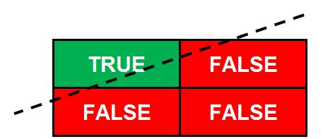
However, if we have a boolean operator ‘XOR’, which stands for ‘Exclusive OR’, where to get True we need one expression to be True while the other is False. Here if both expressions are true the result is false, and if both are false the result is false. Thus if one is true and the other is false, we will get a true. Now when we create the truth table, we can notice that this problem is not linearly separable.

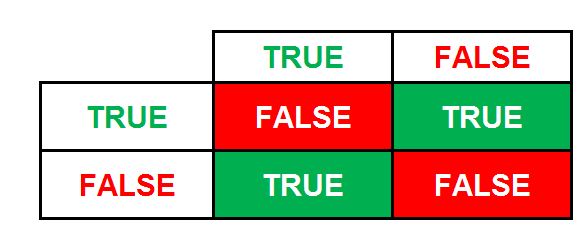
(i.e. for example, A is Age=25 and B is Balance=50; then if Age is not 25 and Balance is 50, then true; Age is 25 but balance is not 50, then true; both Age and Balance being 25 and 50, then false; and when Age and Balance are not 25 and 50, then false).

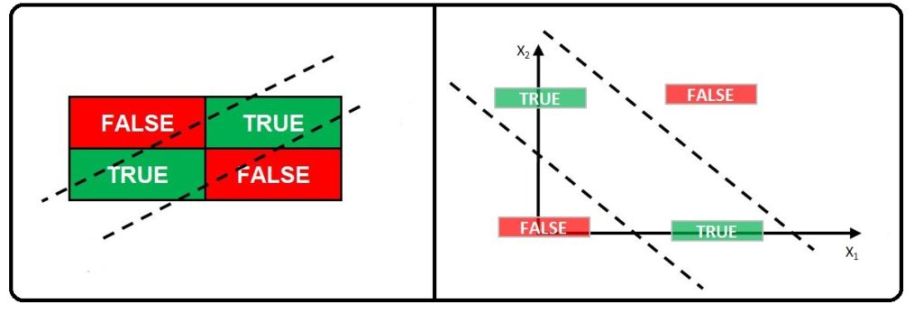
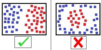
As the Trues and Falses are not on one side, we cannot create a line which will classify them successfully. For this, we need to create two separate lines which will cause the Trues to lie in the middle of the two lines and the Falses on the other sides.

Thus a single neuron cannot solve such a simple boolean operation. To solve such a problem we require adding another neuron, and this takes us to Phase 2 of artificial neural networks, where we learnt to stack and bind these neurons together, creating multilayer perceptrons which can perform more complicated tasks and can handle non-linearly separable data.

Deep Neural Networks (multilayer perceptrons)

XOR Problem

When we use more than one layer/level of perceptrons, then such a network is called a deep neural network. The term ‘Deep Learning’ comes from here, referring to networks that have hidden layers. To solve the XOR problem we will go for a three-layer model rather than the two-layer model used above. Here we will have the input layer and output layer which we had above. In addition to this, we will have two additional perceptrons in the hidden layer, which will lie between the input and output layers. We never directly see the workings of the hidden layer, and that is why they are called so: we only see what we input and what we get as output, while the rest of the data processing is done in these hidden layers.

If we try to solve the XOR problem, this time using more than one layer of perceptrons, we can be successful in correctly classifying the problem.

If we add one layer to the neural network that we had created previously, then we will have two inputs and two neurons in the hidden layer, where one can solve the logical ‘or’ (||) while the other perceptron is the reverse of the logical ‘or’ (||), or we can say it is a ‘not and’ (!&&). Here each input is sent to both perceptrons, and the result is then provided to the perceptron on the output layer, which performs a logical ‘and’. Therefore, if we want True in the output, the first neuron will solve True ‘or’ while the second neuron will find True ‘not and’, and their output will provide us with a True XOR, as these are the only scenarios where ‘or’ and ‘not and’ are both True. Therefore, when both of them are true and they reach the output layer perceptron which performs a logical ‘and’, and as they are both True, the output perceptron outputs True.

For example, we have as input x1: B and x2: A. The input first reaches the first perceptron of the hidden layer, which acts as an ‘or’ operator. As we have AB, which falls under True ‘or’, as for being otherwise the input should have been BB (the four possible combinations being AA, AB, BA, BB), this perceptron is able to remove BB. However, to find the right answer we also require isolating AA, and for this we use the second perceptron. When the input AB reaches the second neuron of the hidden layer, which performs ‘not and’, it finds that it indeed is ‘not and’, as for being otherwise the input should have been AA. Together they are able to eliminate AA and BB. The output from both these perceptrons reaches the output layer perceptron, which performs the logical ‘and’. For producing True it requires ‘True and True’. As the output from both the perceptrons of the hidden layer is True, we get a True in the output, and we are able to solve the XOR problem by adding a layer of perceptrons.

Practical Exercise

If we have denoted True as 1 and False as 0, and we have the following dataset, then we can build a multilayer perceptron.

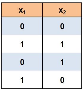
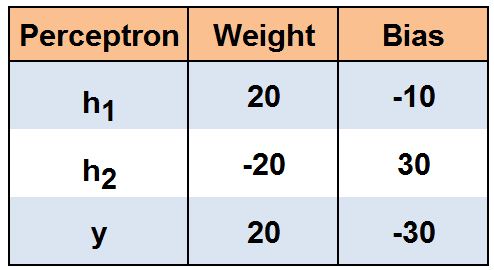
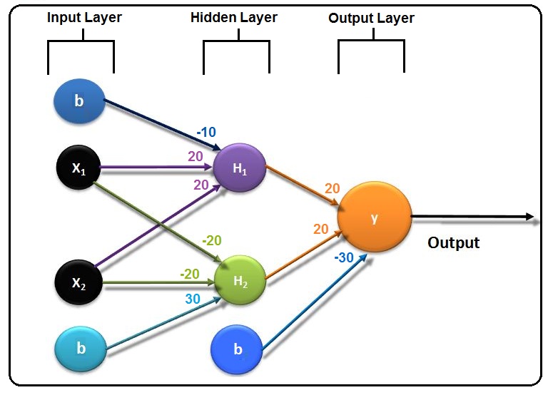
We use a three-layer model wherein the hidden layer we will have two perceptrons, h1 and h2, and another perceptron y in the output layer. We provide the following weights and bias to these perceptrons.

We can now visualise a three-level neural network.

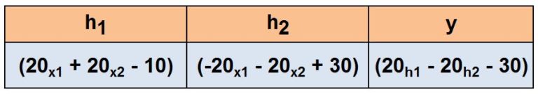
For each perceptron, we will have the following calculations.

For the four data entries, we will multiply the data by the weights and add the bias. As an activation function, we take a very simple step function, where a negative value outputs 0 while a positive value outputs 1. Using the weights, bias, and activation function, we get the following results.

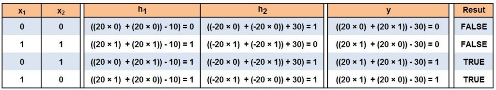
We can see that for 0,1 and 1,0 we are able to get True as the result. Thus the idea behind a Multilayer Perceptron is linking multiple perceptrons together in order to solve non-linearly separable and very complex problems. Also, it is important to understand that so far we have discussed the feedforward process, where all the connections are in one direction without any cycle. In Feedforward, the data from the input unit is passed to the next layer of the unit, and after due computation, the result is passed to the next layer, and so forth, until the results are computed by the output layer.

Backpropagation (Backward Propagation of Errors with Gradient Descent)

In reference to how the human brain works, it was mentioned earlier that to teach a kid the difference between apples and oranges, we can provide them with a lot of different images and the right answer, so that the brain can adjust accordingly each time it gives a wrong answer, and can finally learn to identify the difference between the two fruits.

A concept on similar lines is used in Backpropagation (Backward Propagation of Errors), which was the second major development in Phase 2 of the evolution of Artificial Neural Networks that caused its resurgence. The idea behind Backpropagation is that we initially provide random weights and bias to the neural network and let it complete one iteration, and once complete, we compare the results of the neural network with the actual results, and depending on the magnitude of the error, we tweak the weights and biases of the different perceptrons in order to get better results.

It is important to understand that, unlike the traditional modelling techniques learnt so far, Artificial Neural Networks work more like a black box, as we don’t exactly know how they reach the desired result, which makes it very tough to make an informed decision about tweaking the algorithm to get better results. In the above example, we were able to know what each perceptron was performing and how together they were able to solve an XOR problem; however, when we have hundreds of features, perceptrons, and layers, it becomes impossible to understand what happens inside the hidden layers of the model.

Thus we can only tweak the weights and biases based on the error until we get a combination of those weights and biases which provides us with the best results. Thus, after calculating the error, the model runs backwards, updating the weights and bias of each layer (hence the name backpropagation), and then runs again and calculates the error, repeating the process until the error is minimized.

So far we have discussed the basic process of the working of neural networks, where we input vectorised data, and this data is passed from one layer to another. At each level we perform a matrix operation where we multiply the input by the weight, add a bias term, and apply an activation function to the outcome, then pass it to the next layer, which performs similar calculations. The output from the last layer, known as the output layer, provides us with a prediction, which is then used to compute the error by finding the difference between the actual and predicted value.

This error value is then used to compute the partial derivative with respect to the weight and bias in each layer. This is done from the output layer to the input layer, i.e. it is done recursively, and through this we are able to update the weights and biases and again run forward with the updated weights and biases, computing the error and repeating the process until the minimum error is found. Thus we update the weights and biases through backpropagation in order to decrease the error in the output; however, each iteration can take a lot of time, especially when we have a lot of hidden layers and a number of neurons in each layer, and this brings us to the reason why Phase 2 ended.

For an in-depth understanding of backpropagation, see the supporting article on Artificial Neural Networks Backpropagation

Computational Cost

As discussed at the beginning of this article, the progress of neural networks halted even after the discovery of the multilayer perceptron architecture and backward propagation. This was mainly due to the lack of processing power, as this network could become very complex very easily. For example, if we have two inputs, 0 and 1, then we will be having four combinations of these variables: 00, 01, 10, 11. Ideally, we should have four neurons in the hidden layer, where each can decode one of these combinations. However, if we have a hundred variables, this would mean that we would require 2¹⁰⁰ neurons in the hidden layer to successfully come up with predictions. Thus, because of this architecture, the neural network can become extremely complex, and in more advanced stages, where we have multiple hidden layers with each hidden layer specialising in identifying a key pattern, the process, combined with backpropagation, becomes extremely complex. This caused an end to Phase 2, and it was only recently, with the advent of high-processing units, that ANN was reborn.

Activation Function

We discussed the step method briefly and have explored the sigmoid activation function in detail; however, there are many types of activation functions that can be used, each with their own characteristics.

Step function

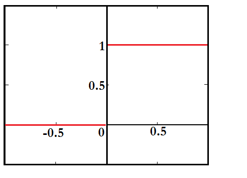
Also known as the Transfer function, it is the most basic type of activation function. Here the threshold is set at zero, where when the value of the output is more than 0 the neuron produces 1 (i.e. the neuron is activated), while if the value of the output is less than 0 the neuron produces 0 (i.e. the neuron does not fire and is not activated). However, this method only works if we have a binary classification problem and is rarely used.

Linear Function

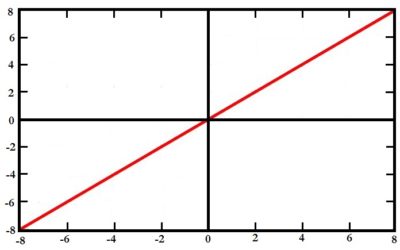
In this method, the output value is passed through the next layer without manipulating it. Here the function is nothing but a straight line, where the value produced by the activation is proportional to what is produced in the output. However, it suffers from a major drawback, which is that it has no upper or lower bound, and most importantly it doesn’t introduce any non-linearity; if all the layers are activated by a linear function, then the activation function of the output layer is nothing but a linear function of the inputs of the first layer. This way, having multiple layers becomes meaningless, and this causes a potential problem.

Sigmoid Function

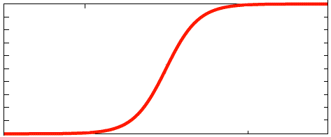
Discussed in detail so far, the sigmoid/logistic activation function is a squashing function where the output is made to lie between 0 and 1, unlike the linear function where the values can lie anywhere between −infinity and infinity. Also, it introduces non-linearity to the network and increases perpetually with bigger values, providing higher activation results. However, despite its advantages, it suffers from a problem called ‘vanishing gradients’. If we look at the function in the graph, we can see that at both ends, the y values respond less to changes in x. This means when running backpropagation, if the activation value is at either end of the graph, the gradient produced will be very small, and this restricts any major update in the weights from happening.

Hyperbolic tangent (Tanh) Function

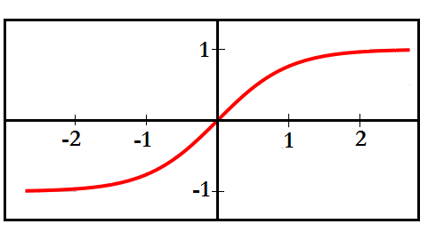
It is among the most commonly used activation functions. Here, unlike the sigmoid function, which doesn’t have 0 as its centre, the hyperbolic tangent function squashes the output between −1 and 1, providing steeper gradients, thus making backpropagation more effective. Like the sigmoid function, it introduces non-linearity to the network; however, it suffers from the problem of vanishing gradients.

Rectified Linear (ReLU) Function

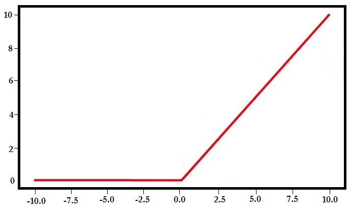
It is the single most popular activation function widely used today. It has a lower limit of zero, where for any negative value a zero is allocated; however, it has no upper bound and can go to infinity, making the activation ‘blow up’. ReLU introduces sparsity in the network, which means that 0 is simply allocated when the value is negative; this produces sparsity of the activation, which saves processing time, as unlike sigmoid or tanh, where each activation is processed, here only those that are non-zero are processed. ReLU also introduces non-linearity in the network and doesn’t suffer from the diminishing gradients problem; however, it suffers from the problem of ‘dead neurons’, where, because of the flat horizontal line in the graph for neurons producing negative values, during backward propagation the gradients for such neurons can go towards 0, making them resistant to any changes in the error, and due to the gradient being low, they become non-responsive to backpropagation, causing the ‘dying ReLU’ problem.

This problem is solved by using variations of ReLU, such as Leaky ReLU, PReLU, Maxout, etc.

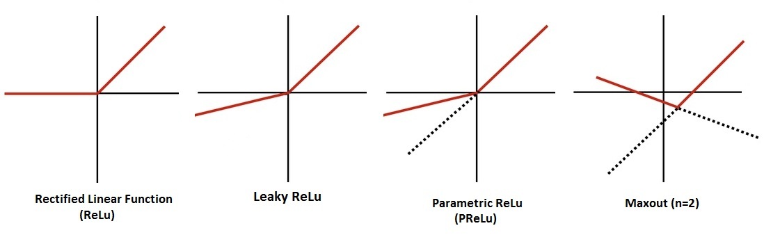
In Leaky ReLU we introduce a small slope, i.e. a non-horizontal component to the previously horizontal line, making Y=0.01x for x<0. Thus we allow a small non-zero gradient when the neuron is not active. Another variant of Leaky ReLU is Parametric ReLU (PReLU), where the idea of Leaky ReLU is taken further by making the coefficient of leakage a parameter that is learned along with the other neural network parameters. Here Y=ax for x<0. We also have another function known as Maxout, which is a combination of ReLU and Leaky ReLU.

ReLU is the most used activation function; however, it should be used in the hidden layers, and the Linear function should be used at the output layer in the case of Regression problems, while SoftMax (a squashing function) should be used in the output layer when dealing with classification problems.

Thus we have a lot of activation functions that can be used while building a neural network. One must remember that activation functions are very important, as without applying a function the output from each layer will be a simple linear function, which eventually makes our neural network model behave like a regression model. As mentioned at the beginning of this article, we want our neural network model to behave like a human brain, which can work with any kind of data, thus making them Universal Function Approximators, meaning that they can represent features originating from various kinds of data (audio, video, images, etc.) and can compute and learn any kind of function. To do so we require our model to be complex enough to not only compute linear functions but to learn more complex functions, and for that we introduce different activation functions and add a lot of hidden layers. Also, as mentioned above, activation functions such as Tanh and ReLU provide the much-needed non-linearity in the model in order to make the model differentiable, allowing backpropagation to function properly.

Artificial Neural Networks are the stepping stone for understanding the workings of various models related to Deep Learning. ANN provides very accurate answers; however, it is computationally expensive during the training period, while being relatively fast during the testing phase, and should be used especially when solving very complex problems.