// shared: regression & classification

Regularized Regression Algorithms

There are many modern regression approaches that can be used rather than the classic Linear or Logistic Regression. As discussed in Linear Regression, we use the Ordinary Least Squares (OLS) method to estimate the unknown parameters in the linear regression model; however, this is a very old method, and more modern and sophisticated methods, such as regularization methods, can be used for building linear and logistic models.

It is important to understand from the beginning that regularization methods do not improve the process of learning these parameters, but rather help with the generalization part (i.e. help increase the accuracy of the model when working with unseen data), which they do by penalizing the complexity of the model (complexity is caused by overfitting, where the model ‘memorizes’ the patterns in the data too much and makes assumptions when there are none).

Thus, to keep the model away from including noise and other peculiarities during generalization, regularized regression models can be used. The single biggest reason for a model to get very complex is its reliance on too many features, and to deal with data that is in very high dimensions, such advanced regression models can be used.

Limitations of OLS

The standard formula of a simple linear regression model is Y = B0 + B1X1 + E, where B0 is the intercept, X1 is the independent variable, B1 is the coefficient, and E is the error term. By using this equation we get Y, which is our predicted value, and using Y we get to know E, which is the value that needs to be corrected for the prediction error between the observed and predicted value. This error term is very important, as every predicted value will not be correct and will be different from the actual value, and the error term is used to correct this difference. This is where OLS comes in, as it tries to minimize this difference, which it does by finding the regression line that minimizes this error (the software tries various regression lines in the backend and finally selects the regression line that gives the least sum of squared error, i.e. the difference between predicted and observed values).

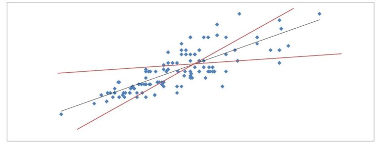
Thus, OLS, if calculated visually, is the sum of the distances between each data point and its corresponding predicted data point that lies on the regression line, and the regression line is set where this sum is the minimum.

Till now we have used the sum of squared error to represent the error present in our OLS regression model; however, it is important to further understand this error. Prediction error can be divided into two types: error due to bias, and error due to variance.

To understand these sub-components of error, we have to find the different sources of error. These sources stem from the idea of generalization, which basically involves generalizing based on what we have previously seen onto a new dataset. Thus, when building a model, we don't have one but two goals: how accurate the model is, and how well the model performs on unseen data. Both these concepts are fundamentally opposed to each other, as when we try to increase the model's accuracy, we decrease its generalizing power, and when we try to make the model more ‘generalization friendly’, we lose accuracy.

To put this in context, let us say we have a dataset where the Y variable has two categories: Rich, Poor. We have 100 demographic independent features, ranging from the city they live in to whether they wear spectacles or not. If we were to increase the accuracy of our model, we could literally make our model memorize the patterns in our dataset, which would end up memorizing patterns that, in real life, make no sense in indicating the financial situation of a person, such as whether males have a moustache or not, or their taste preferences, etc. This leads to the problem of overfitting, where we find too many patterns, including matching patterns that exist by chance, perhaps due to noise in the data. Thus, if we have very high complexity, it means we have very high variance.

To improve the situation, let's say we take only one feature. This will lead to very high bias and very low variance, and this will also have its own set of problems, as by having only one feature to generalize from, we make a big assumption about our data. Let's say we generalize our data on the basis of the region of the country; this is a very big assumption, and it will result in very low model accuracy, causing our model to underfit.

To increase the model's accuracy, we then make our model more complex by adding another feature, say their academic qualification. By adding one more feature we reduce the bias and increase the variance, but if we keep going with this and keep adding features, we will reach a point where we started, i.e. having very high variance and low bias. Thus, a tradeoff exists between them, and we have to find the ‘sweet spot’ where the model is neither too biased (causing underfitting, making the model come up with an extremely simple solution that may not be useful) nor has too much variance (causing overfitting, where patterns in the dataset are ‘memorized’ that may not actually exist and may be there by chance).

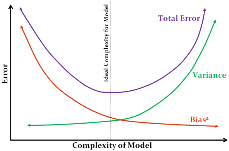
Mathematically, the mean squared error of the estimator is equal to the square of the bias plus the variance. If we look at the image above, we can see how, with increasing complexity of the model, the bias decreases and vice versa, with the optimal point lying somewhere in between, where the total error becomes minimum and the increase in bias is equivalent to the reduction in variance.

Now the question is, why is OLS not the best method? Well, because according to the Gauss-Markov Theorem, ‘among all unbiased estimates, OLS has the smallest variance’. This means that OLS estimates have the smallest mean squared error with no bias. However, we can have a biased estimate that has an even smaller mean squared error, and for that we can use shrinkage estimators, where the regression equation's coefficients (Beta-K) are replaced with Beta′-K, which produces a value lower than the original coefficient.

β′_k = 1 / (1 + λ) × β_k

Here, the original coefficient is multiplied by a term, which is 1 divided by (1 + lambda). So if lambda is 0, we get the original coefficient back; however, if the parameter gets large, the output value gets lower and approaches the minimum value, which is zero. This lambda is the shrinkage estimator, which, if set correctly, provides a better (lower) mean squared error. To find the value of lambda, we use a formula, and without getting into the nitty-gritty of the mathematics behind it, what it does is find whether a coefficient is relatively large compared to its variance, causing the output (lambda) to be smaller. This lambda can thus either kill a coefficient (making it zero) or keep the coefficient but shrink it.

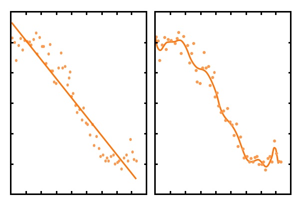
Below we can see how the complexity of the model increases when creating an OLS Polynomial Regression Model using 15 features (right) rather than just one feature (left). An increase in the number of features increases the complexity of the model, and it also starts getting influenced by less important features and tries to fit even the smaller deviations. Consequently, the value of coefficients also increases with the increase in model complexity.

To control the complexity of the model and counter multicollinearity, we use other regression models that can perform regularization. In this article, three types of regularized regression modeling techniques are explored: Ridge Regression, Lasso Regression, and Elastic Net Regression.

Ridge Regression

Ridge Regression can be used to create a regularized model where constraints are put on the algorithm to penalize coefficients for being too large, thus preventing the model from becoming too complex and causing overfitting. In very simple terms, it adds a penalty α‖w‖ to the equation, where w is the vector of model coefficients, ‖·‖ is the L2 norm, and α is a tunable free parameter. This makes the whole equation look like:

β̂ = argmin_β ‖y − Xβ‖² + λ‖β‖²

Here the first component is the least squares term (loss function) and the second is the penalty. In Ridge Regression, L2 regularization is performed, which adds a penalty equivalent to the square of the magnitude of the coefficients. Thus, under Ridge Regression, an L2 norm penalty, which is α∑ⁿ_i=1w²_i, is added to the loss function, thereby penalizing the betas. As the coefficients are squared in the penalty component, this has a different effect than the L1 norm used in Lasso Regression (discussed below). The choice between Ridge and Lasso (and the Elastic Net that blends the two) is set by a separate mixing parameter, often called the L1 ratio: a value of 0 gives pure Ridge, 1 gives pure Lasso, and anything in between gives Elastic Net. Note that this mixing parameter is distinct from the penalty strength described above - confusingly, some libraries also call one of these ‘alpha’. In R’s glmnet, alpha is the mixing parameter, whereas in Python’s scikit-learn alpha is the penalty strength and the mix is set by a parameter called l1_ratio.

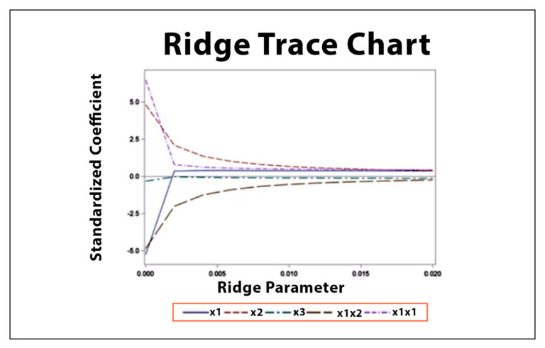
This leaves us with the most crucial aspect, which is deciding the value of the tunable parameter lambda. If we use a very low lambda value, the output will be the same as OLS Regression, and thus not much generalization will take place; however, if we take too large a value for lambda, it will generalize too much, pulling the coefficients of too many features down towards extreme minimum values (i.e. towards 0). Statisticians use methods such as the Ridge Trace, a plot that shows ridge regression coefficients as a function of lambda, and select the value of lambda where the coefficients stabilize. We can use methods such as cross-validation along with grid search to find the best value of lambda for our model.

Ridge uses L2 regularization, forcing coefficient values to be spread out more equally, and doesn't shrink any coefficient to the extent that it becomes 0; however, L1 regularization forces the coefficients of less important features to be zero, and this leads us to Lasso Regression.

Note: Ridge Regression may or may not be considered a Feature Selection method, as it only reduces the size of coefficients and, unlike Lasso, doesn't make any variable obsolete, which can be said to be a proper Feature Selection method.

Lasso Regression

Lasso works the same as Ridge but performs L1 regularization, which adds a penalty α∑ⁿ_i=1|w_i| to the loss function, thereby adding a penalty equivalent to the absolute value of the magnitude of coefficients, rather than the square of the coefficients (used in L2), making weak features have zero as their coefficient. In a way, by using L1 regularization, Lasso performs automatic feature selection, where features with 0 as the value of their coefficient are dropped. Again, the value of lambda is important, as if the value is too large, it ends up dropping a lot of variables (by causing coefficients that are a bit small to become 0), making the model too generalized and causing it to underfit.

Using the correct value of lambda, we can have a sparse output where certain unimportant features are given 0 as a coefficient; these variables can be dropped, and the variables with non-zero coefficients can be selected, thus facilitating feature selection for modeling.

Elastic Net Regression

Elastic Net is a combination of Ridge and Lasso Regression, as it uses both L1 and L2 regularization. It is useful when there are multiple features that are correlated with each other.

β̂ = argmin_β(‖y − Xβ‖² + λ₂‖β‖² + λ₁‖β‖₁)

We can see in the above equation how both L1 and L2 norms are used to regularize the model.

Thus, these regularized regression models can be used to find the correct relationship shared between the independent and dependent variables by regularizing the independent variables' coefficients. They help curb the menace of multicollinearity. Applying regularization to certain regression models can be problematic where the independent features are non-linearly related to the dependent variable. To counter this problem, we can transform the features so that linear models such as Ridge and Lasso can still be applicable, such as by using polynomial basis functions with linear regression, where such transformed features allow the linear model to find the polynomial or non-linear relationships in the data.