// application · python

Descriptive Statistics in Python

Various Descriptive Statistics have been explored in the Theory section. In this blog, we will be discussing how to apply those basic statistics to datasets using Python. In the theory section, we covered four types of basic descriptive statistics and all those will be covered in this blog. Those four topics are:

• Measures of Frequency
• Measures of Central Tendency
• Measures of Variability
• Measures of Shape

These descriptive statistics act as the foundation for more complex analysis. This blog will explore ways in which Python can be used to calculate mean, variance, standard deviation etc, which will act as the building blocks of the statistical analysis of our data. Various visualizing methods such as representing the outcomes graphically using graphs and pie charts will also be explored. Various uni and bivariate analysis will also be explored here as different methods of univariate and bivariate analysis are performed using these basic statistical concepts only.

Preliminary Libraries

Note that certain preliminary libraries are to be imported in Python to work on arrays and data frames for statistical analysis.

To do so, we first will import the preliminary libraries such as numpy and pandas. Both these are very important packages where Numpy is used for operations on arrays whereas pandas is used for performing various operations on DataFrames. Other preliminary packages involve matplotlib which will help us in creating various types of graphs.

import numpy as np
import pandas as pd
import matplotlib.pyplot as plt
%matplotlib inline

Here %matplotlib inline is used to see the graphs in the output itself.

Measures of Frequency

Under Measures of Frequency, the data can be analysed by creating frequency tables.

Import Dataset: We will be working on a hypothetical Diamond dataset to study the relationship between Price and Color of the diamonds. This diamond dataset is a dataset of the diamonds that were sold in a shop. We first start by importing the dataset.

DiamondData = pd.read_excel("C:/Users/user/Desktop/Data Sets/DiamondData.xls")
DiamondData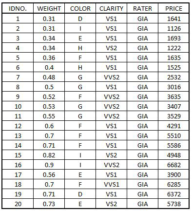

Show full table ▾

Grouping Data

We now use the groupby command to get the total price by Color.

g = DiamondData.groupby('COLOR')['PRICE'].sum()
g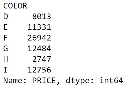

Univariate Analysis using Measures of Frequency

Various kinds of Univariate Analysis concerning a categorical variable can be performed using Measures of Frequency.

Bar Graph: To show this output graphically, we will plot a bar graph for the same. This is done by plotting a bar graph for Price in ascending order. Here figsize is used to define the size of the figure (length, breadth).

BarGraph = g.sort_values().plot(kind="bar",figsize=(8,8),title='Bar Graph for Diamond Data',legend=True,fontsize=12,color='b')
BarGraph.set_xlabel("Color",fontsize=12)
BarGraph.set_ylabel("Price",fontsize=12)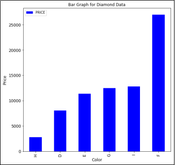

Now we will consider another dataset, which will be a sample customer database. Measures of frequency will be applied to this data in order to study the distribution of customers based on the country of residence.

Import Dataset: We will begin with importing the dataset and then make the frequency table. Here we import a csv file that has the required data.

FreqData1 = pd.read_csv('C:/Users/user/Desktop/Data Sets/FreqData1.csv')
FreqData1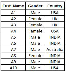

Frequency Table: We use the pd.crosstab function to generate frequency tables.

freq_Country = pd.crosstab(index=FreqData1["Country"],columns="Count")
freq_Country

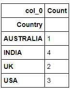
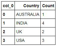
In order to make the data look neat/flat, we use reset_index(). This helps in reducing the extra space found in the table.

Freq_Country =freq_Country.reset_index()
Freq_Country

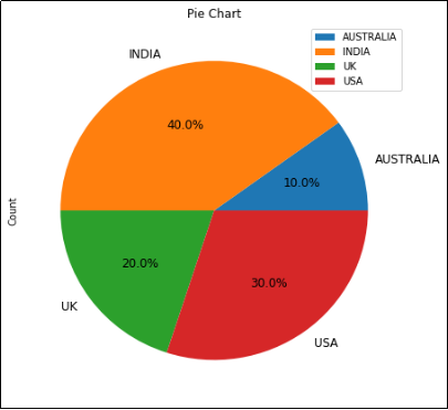
Pie Chart

In order to represent this data graphically, we will make use of a pie chart which acts as a kind of univariate analysis.

Pie_Chart = freq_Country.plot(kind="pie",y='Count',autopct='%1.1f%%',title='Pie Chart',fontsize=12,figsize=(7,7))

Bivariate Analysis using Measures of Frequency

Various kinds of bivariate analysis can be performed using Measures of Frequency. Here unlike before, we consider two categorical variables for our analysis.

Import Dataset: Now, we will discuss bivariate analysis for which we will again consider the dataset that has been used earlier (customer database). We first import the dataset.

FreqData2 = pd.read_csv('C:/Users/user/Desktop/Data Sets/Demographics_of_customers.csv')
FreqData2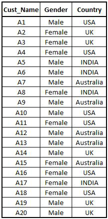

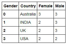
Show full table ▾

Frequency Table: As we are performing bivariate analysis using Measures of Frequency, therefore unlike before, we create a frequency table by considering two categorical variables.

FreqData2_table = pd.crosstab(index=FreqData2["Country"],columns=FreqData2["Gender"])
FreqData2_table.reset_index()

Stacked Bar Chart

However, as we are performing bivariate analysis using Measures of Frequency, we will also take another variable, ‘gender’, as a parameter for our analysis. To perform a visual bivariate analysis using Measures of Frequency, we create a Stacked Bar Chart to represent the data.

Stacked = FreqData2_table.plot(kind="bar",figsize=(8,8),stacked=True,title='Stacked Bar Chart',fontsize=12)
Stacked.set_ylabel("Count",fontsize=12)
Stacked.set_xlabel("Country",fontsize=12)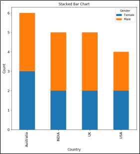

These univariate and bivariate analyses using Measures of Frequency help us in understanding the data. We now can proceed with the application of other Descriptive Statistics.

Measures of Central Tendency

Measures of Central Tendency tells us the way in which a group of data clusters around the central value. The main three measures are: Mean, Median and Mode. Mean is the average value of the data. Median is the middle value when data is arranged in ascending or descending order while mode is the most occurring value.

Import dataset: To calculate these values, we first import an arbitrary dataset having the height of 20 people.

HeightData1 = pd.read_excel('C:/Users/user/Desktop/Data Sets/Height_Data1.xls')
HeightData1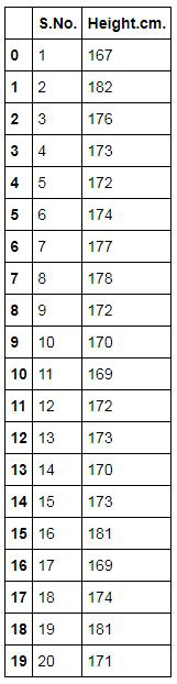

Show full table ▾

Mean, Median and Mode

Mean:

HeightData1['Height.cm.'].mean()

Median:

HeightData1['Height.cm.'].median()

Mode: We need to first import the mstats package to calculate mode.

import scipy.stats.mstats as mstats

def mode(x):
    return mstats.mode(x, axis=None)[0]

We now can use this package to calculate the mode of the variable ‘Height’.

mode(HeightData1['Height.cm.'])

Effects of Outlier on Measures of Central Tendency

An outlier is a value of a dataset which is very different from the other values, i.e. the difference between an outlier and other values is big. Outliers affect the mean of the dataset (which is a measure of central tendency) which can cause wrong analysis of our dataset. We can understand this effect using Python.

Import Dataset: For example, we have a dataset that has the same observations as mentioned above (heights of 20 people), however this time the 17th observation is an outlier.

HeightData2 = pd.read_excel('C:/Users/user/Desktop/Data Sets/Height_Data2.xls')
HeightData2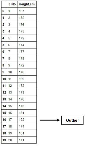

Show full table ▾

Now if we calculate mean, median and mode we will find that it has affected the value of the mean.

Mean (when the dataset has an outlier):

HeightData2['Height.cm.'].mean()

Median (when the dataset has an outlier):

HeightData2['Height.cm.'].median()

Mode (when the dataset has an outlier):

def mode(x):
    return mstats.mode(x, axis=None)[0]

mode(HeightData2['Height.cm.'])

Earlier, the mean was 173.7, and when an outlier was present it became 174.85. Therefore we see that only Mean gets affected by the presence of an outlier while Median and Mode remain the same. Right now the difference in the means is not so much as we have a small dataset with only one small outlier however when we are dealing with large datasets, the difference in means will be very significant. Thus as discussed in the theory section, the mean has a disadvantage of being adversely affected by outliers.

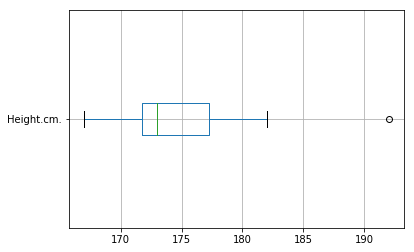
Methods of Identifying Outlier: One can identify an outlier by plotting a box plot. Box plot represents the second and third quartiles. The dot in a box plot is an identification mark for an outlier. Here in the code, a vert command can be adjusted to make the boxplot to be in a vertical or horizontal format.

HeightData2.boxplot(column="Height.cm.",vert=False)

With this, we cover the three Measures of Central Tendency.

Measures of Variability

Measures of variability are calculated to see how ‘spread out’ the data is. There is a possibility that two different datasets have exactly the same mean but have a different level of variance. Therefore, if we just take mean into account for our analysis then we will come up with wrong interpretation of our datasets. To explain this, we will take two datasets of scores of two classes, Class A and Class B, having the same mean and calculate the Measures of Variability: Range, Variance and Standard Deviation.

Creating Datasets: First, we will create these datasets in Python.

Scores_A = [20,18,12,18,16,20,13,19,16,17]
Scores_B = [9,10,17,18,17,19,20,20,20,19]
Scores_A =  pd.DataFrame(Scores_A)
Scores_B = pd.DataFrame(Scores_B)

Note that we converted Scores_A and Scores_B to data frames as functions such as mean, variance etc can be directly applied to data frames. Whereas, for lists, one has to define the functions to calculate mean etc.

Range

In range we calculate multiple metrics such as the minimum value, maximum value, quartiles etc.

Minimum Value: We can calculate the minimum value of the datasets using the min() function. Minimum Value of the dataset Scores_A:

Scores_A.min()

Minimum Value of the dataset Scores_B:

Scores_B.min()

We can similarly use the height dataset and find the minimum value of the variable ‘Height.cm.’ This time we use the min function.

min(HeightData1['Height.cm.'])

Maximum Value: Maximum Value of the dataset Scores_A:

Scores_A.max()

Maximum Value of the dataset Scores_B:

Scores_B.max()

Maximum value of the variable ‘Height.cm.’ in the Height dataset:

max(HeightData1['Height.cm.'])

Quartiles

We can find the quartiles of both the datasets created above.

Quartiles for dataset Scores_A:

Scores_A.quantile(q=(0.25,0.5,0.75,1))

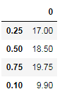
Quartiles for dataset Scores_B:

Scores_B.quantile(q=(0.25,0.5,0.75,1))

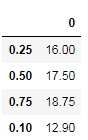
Quartiles for the variable ‘Height.cm.’ in the Height dataset:

Quantiles = [HeightData1['Height.cm.'].quantile(0.25),
             HeightData1['Height.cm.'].quantile(0.50),
             HeightData1['Height.cm.'].quantile(0.75),
             HeightData1['Height.cm.'].quantile(1)]

Variance

The variance is among the most important Measures of Variability. We find the variance of both the above-created datasets.

Variance for dataset Scores_A:

Scores_A.var()

Variance for dataset Scores_B:

Scores_B.var()

Variance for the variable ‘Height.cm.’ in the Height dataset:

HeightData1['Height.cm.'].var()

Means v/s Variance

We first calculate the mean of both the datasets, Scores_A and Scores_B.

Mean of Scores_A:

Scores_A.mean()

Mean of Scores_B:

Scores_B.mean()

We find that the mean of both the datasets, Scores_A and Scores_B, is the same at 16.9. Thus we see that even though the two datasets have exactly the same mean, they have a different level of variance. In our example, the scores by Scores_B are more spread out.

Standard Deviation

The most famous and commonly used Measure of Variation.

Standard Deviation for dataset Scores_A:

Scores_A.std()

Standard Deviation for dataset Scores_B:

Scores_B.std()

Standard Deviation for the variable ‘Height.cm.’ in the Height dataset:

HeightData1['Height.cm.'].std()

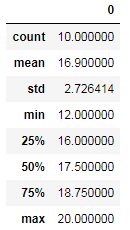
Summary Statistics

One can also use the describe function for summary statistics which is the equivalent of Summary in R.

Scores_A.describe()

Measures of Shape

In the Theory section of Descriptive Statistics, Measures of shape were explored in order to see how our dataset is distributed, i.e. whether the distribution is normal or skewed. To find this, we either plot the dataset or calculate the level of skewness or kurtosis.

If our dataset has a bell-shaped curve, then our dataset is normally distributed. Here, the mean, median and mode are equal and all lie in the middle.

We can calculate or visualize skewness which tells us to what degree our data is skewed. If most of the observations lie on the left side of the graph then it is called negatively skewed data, where the mean < median. The vice-versa of this would be called positively skewed data. Kurtosis is based on the height of the curve. A lot of modeling algorithms require the dataset to be normally distributed. Therefore, we use measures of skewness to check for normality. If the dataset is skewed then we transform the variable to normalize the dataset. (This is discussed in detail in the Feature Engineering blog.)

We take the scores data (used above) to measure skewness and kurtosis.

Calculating Skewness

The measure of Skewness can be calculated by using Python. By default, Python uses a method called Moment method.

Scores_A.skew()

Calculating Kurtosis

Kurtosis can be calculated by using Python. By default, Python uses a method called Fisher method.

Scores_A.kurt()

Normal Distribution

Visually, anything which doesn’t look like a normal distribution is either skewed or has kurtosis, or is bimodal or multimodal. Therefore it is important to know how a normally distributed dataset looks like.

Import Dataset: We import a hypothetical dataset having exam scores of students where the mean = mode = median.

Marks_Scored = pd.read_excel('C:/Users/user/Desktop/Data Sets/Marks_Scored.xls')
Marks_Scored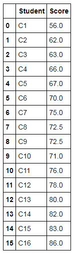

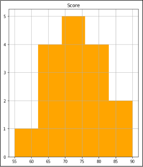
Show full table ▾

Plot Histogram: We now plot a histogram on this dataset to see the distribution of data visually.

Marks_Scored.hist(column="Score",figsize=(6,7),color="orange",bins=5,range=(55,90))

Plot Line Graph: To have more clarity, we use a line graph to see if the distribution of data is bell-shaped or not.

Marks_Scored.plot(kind="density",figsize=(6,7))

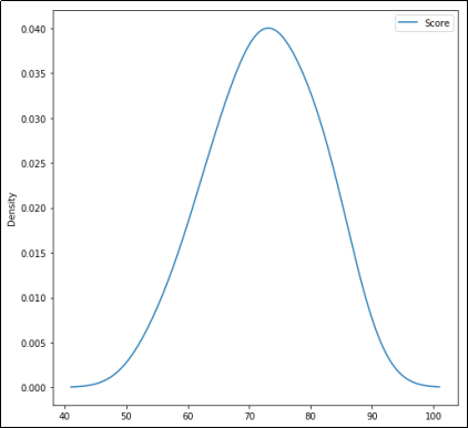
We can see that the distribution forms a bell-shaped curve which tells us that the dataset is normally distributed. Similarly, we can plot other datasets and if they show similarity to the shapes discussed in the Measures of Shape then they may not be normal.

In this blog, we applied the concepts explored in the theory part of Descriptive Statistics. Python is a powerful tool and can be used for univariate and bivariate analysis using various descriptive statistics. It provides tools to perform various statistical calculations along with visualising the dataset. In the next blog, the concepts of Inferential Statistics explored in the Theory section have been put to use using Python.