// application · r

Descriptive Statistics in R

Various Descriptive Statistics have been explored in the Theory section. In this blog, we will be discussing how to apply those basic statistics to datasets using R. In the theory section, we covered four types of basic descriptive statistics and all those will be covered in this blog. Those four topics are:

Measures of Frequency
Measures of Central Tendency
Measures of Variability
Measures of Shape

These descriptive statistics act as the foundation for more complex analysis. This blog will explore ways in which R can be used to calculate mean, variance, standard deviation etc, which will act as the building blocks of the statistical analysis of our data. Various visualizing methods such as representing the outcomes graphically using graphs and pie charts will also be explored. Various uni and bivariate analysis will also be explored here as different methods of univariate and bivariate analysis are performed using these basic statistical concepts only.

Measures of Frequency

Under Measures of Frequency, the data can be analysed by creating frequency tables.

Import an excel file to R: We will be working on a hypothetical Diamond dataset to study the relationship between Price and Color of the diamonds. This diamond dataset is a dataset of the diamonds that were sold in a shop. We will first load the package readxl to import an excel file. To load an installed package in R we use the command library.

library(readxl)
DiamondData <- read_excel('C:/Users/user/Desktop/Data Sets/DiamondData.xls')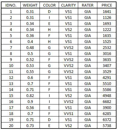

Diamond dataset: 20 rows with IDNO, WEIGHT, COLOR, CLARITY, RATER and PRICE columns — Output: the Diamond dataset.

Grouping Data

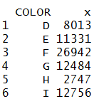
We now use the aggregate command to get the total price by Color.

g <- aggregate(DiamondData$PRICE,by=list(COLOR=DiamondData$COLOR),FUN=sum)
g

Total PRICE summed by COLOR — Output: total price by Color.

Univariate Analysis using Measures of Frequency

Various kinds of Univariate Analysis concerning a categorical variable can be performed using Measures of Frequency.

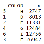
Bar Graph: To show this output graphically, we will plot a bar graph for the same. This is done by plotting a bar graph for Price in ascending order. First, we will use the order command to sort the price in ascending order and use the output to plot a bar graph.

# Order the data by x i.e. Price (summed) i.e x
G1 <- g[order(g$x),]
G1

Diamond price totals ordered ascending by COLOR — Output: price totals ordered ascending.

Plot a bar graph for the above output. Here main is used to define the title of the graph while xlab and ylab are used to label the axis.

barplot(G1$x,col="blue",main="Barplot of Diamond Price by Colour",
xlab="COLOR",ylab="Price",names.arg=c("H","D","E","G","I","F"))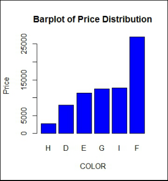

Bar graph of Price by Color, sorted ascending — Output: bar graph of the Diamond data.

Now we will consider another dataset, which will be a sample customer database. Measures of frequency will be applied to this data in order to study the distribution of customers based on the country of residence.

Import a CSV File in R.

FreqData1 <- read.csv("C:/Users/user/Desktop/R - Basic Stats/Data Sets/FreqData1.csv")
View(FreqData1)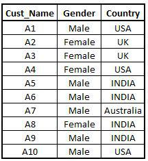

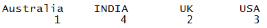
Customer database FreqData1 with Cust_Name, Gender and Country — Output: the customer database.

Frequency Table

Creating Frequency table using table command in R.

table(FreqData1$Country)

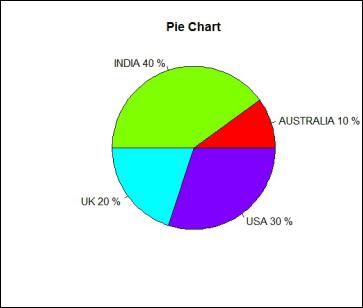
Frequency table of Country counts — Output: frequency table of Country.

Pie Chart

In order to represent this data graphically, we will make use of a pie chart which acts as a kind of univariate analysis.

We use table to create a frequency table for the pie chart. The command prop.table is used to get the percentages for the pie chart. col is used to define the colour. One can also adjust the size of the pie by changing the value of radius.

Pie1 <- table(FreqData1$Country)
pertab <- prop.table(Pie1)*100
pie(Pie1,main="Pie Chart",labels=paste(names(Pie1),pertab,"%",sep=" "),col=rainbow(4),radius=1)

Pie chart of Country share: Australia 10%, India 40%, UK 20%, USA 30% — Output: pie chart of Country share.

Bivariate Analysis using Measures of Frequency

Various kinds of bivariate Analysis can be performed using Measures of Frequency. Here unlike before, we consider two categorical variables for our analysis.

Import Dataset: Now, we will discuss bivariate analysis for which we will again consider the dataset that has been used earlier (customer database). We first import the dataset.

FreqData2 = read.csv('C:/Users/user/Desktop/Data Sets/Demographics_of_customers.csv')
View(FreqData2)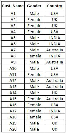

Demographics dataset FreqData2: 20 customers with Gender and Country — Output: the demographics dataset.

Frequency Table

Creating Frequency table for bi-variate dataset using the table command.

table(FreqData2$Gender,FreqData2$Country)

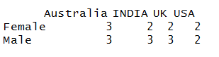
Cross frequency table of Gender against Country — Output: cross frequency table of Gender and Country.

Stacked Bar Chart

However, as we are performing bivariate analysis using Measures of Frequency, we will also take another variable, ‘gender’, as a parameter for our analysis. To perform a visual analysis using Measures of Frequency, we create a Stacked Bar Chart to represent the data. Here beside command is used to define the type of bar chart we require and in case of a stacked bar chart we write beside = FALSE or F. The position of the legend can be specified in the code by adding legend="topright", or "bottom" etc. One can also use the inset command to define the size of the legend box.

Stackplot <- table(FreqData2$Gender,FreqData2$Country)
barplot(Stackplot,beside=F,col=c(2,4),xlab="Country",ylab="Count",main="Stacked Bar Graph",legend.text
=c("Male","Female"),legend="topright",xlim=c(0,4),width=0.6,inset=c(-0.1,1))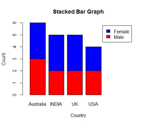

Stacked bar chart of Count by Country, split by Gender — Output: stacked bar chart by Country.

These univariate and bivariate analyses using Measures of Frequency help us in understanding the data. We now can proceed with the application of other Descriptive Statistics.

Measures of Central Tendency

Measures of Central Tendency tells us the way in which a group of data clusters around the central value. The main three measures are: Mean, Median and Mode. Mean is the average value of the data. Median is the middle value when data is arranged in ascending or descending order while mode is the most occurring value.

Import dataset: To calculate these values, we first import an arbitrary dataset having the height of 20 people.

HeightData1 = read_excel('C:/Users/user/Desktop/Data Sets/Height_Data1.xls')
View(HeightData1)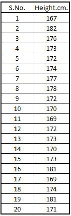

Height dataset of 20 people with S.No. and Height.cm. — Output: the height dataset.

Measures of Central Tendency: Mean, Median, Mode

Mean:

mean(HeightData1$Height.cm.)

173.7

Median:

median(HeightData1$Height.cm.)

173

Mode: As there is no inbuilt function to compute mode of a dataset, we will create the function in the editor window and then run it. This function will be stored in the Global environment and can be used on other datasets as well.

Mode Function

getmode <- function(v) {
  uniqv <- unique(v)
  uniqv[which.max(tabulate(match(v,uniqv)))]
}

Using Function

v <- HeightData1$Height.cm.
result <- getmode(v)
print(result)

172

Effects of Outlier on Measures of Central Tendency

An outlier is a value of a dataset which is very different from the other values, i.e. the difference between an outlier and other values is big. Outliers affect the mean of the dataset (which is a measure of central tendency) which can cause wrong analysis of our dataset. We can understand this effect using R.

Import Dataset: For example, we have a dataset that has the same observations as mentioned above (heights of 20 people), however this time the 17th observation is an outlier.

HeightData2 = read_excel('C:/Users/user/Desktop/Data Sets/Height_Data2.xls')
View(HeightData2)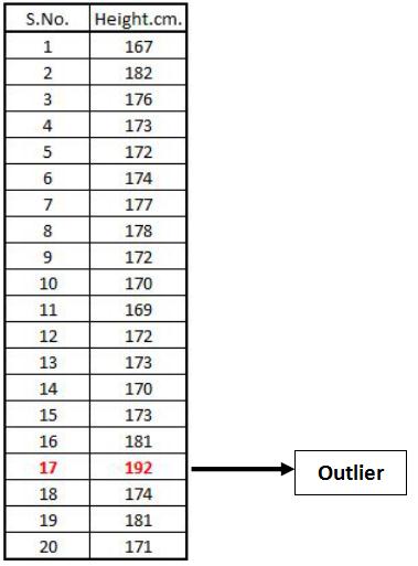

Height dataset where the 17th observation, 192, is marked as an Outlier — Output: the height dataset with an outlier at the 17th observation.

Now if we calculate mean, median and mode we will find that it has affected the value of the mean.

Mean (when the dataset has an outlier):

mean(HeightData2$Height.cm.)

174.85 (More than before)

Median (when the dataset has an outlier):

median(HeightData2$Height.cm.)

173 (Same as Before)

Mode (when the dataset has an outlier):

v <- HeightData2$Height.cm.
result <- getmode(v)
print(result)

172 (Same as Before)

Earlier, the mean was 173.7, and when an outlier was present it became 174.85. Therefore we see that only Mean gets affected by the presence of an outlier while Median and Mode remain the same. Right now the difference in the means is not so much as we have a small dataset with only one small outlier however when we are dealing with large datasets, the difference in means will be very significant. Thus as discussed in the theory section, the mean has a disadvantage of being adversely affected by outliers.

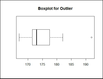
Methods of Identifying Outlier: One can identify an outlier by plotting a box plot. Box plot represents the second and third quartiles. The dot in a box plot is an identification mark for an outlier. (If horizontal = F is used then a vertical boxplot will be generated and the dot at the right end is the outlier.)

boxplot(HeightData2$Height.cm.,horizontal = T,main="Boxplot for Outlier")

Horizontal box plot of Height showing the outlier as a separate point — Output: box plot identifying the outlier.

With this, we cover the three Measures of Central Tendency.

Measures of Variability

Measures of variability are calculated to see how ‘spread out’ the data is. There is a possibility that two different datasets have exactly the same mean but have a different level of variance. Therefore, if we just take mean into account for our analysis then we will come up with wrong interpretation of our datasets. To explain this, we will take two datasets of scores of two classes, Class A and Class B, having the same mean and calculate the Measures of Variability: Range, Variance and Standard Deviation.

Creating Datasets: First, we will create these datasets in R.

Score_A <- c(20,18,12,18,16,20,13,19,16,17)
Score_B <- c(9,10,17,18,17,19,20,20,20,19)

Range

In Range, we calculate multiple metrics such as the minimum value, maximum value, quartiles etc. Unlike Python, R has a Range function which gives you the minimum and the maximum value of a dataset.

Calculating the range of Score_A:

range(Score_A)

12 20

Calculating the range of Score_B:

range(Score_B)

9 20

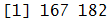
We can similarly use the height dataset:

range(HeightData1$Height.cm.)

167 182

Quartiles

We can find the quartiles of both the datasets created above.

Quartiles for dataset Scores_A:

quantile(Score_A)

Quartiles for dataset Scores_B:

quantile(Score_B)

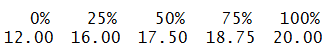
Quartiles for the variable ‘Height.cm.’ in the Height dataset:

quantile(HeightData1$Height.cm.)

Quartiles for Height.cm.: 0% 167, 25% 170.75, 50% 173, 75% 176.25, 100% 182 — Output: quartiles for Height.cm.

Variance

The variance is among the most important Measures of Variability. We find the variance of both the above-created datasets.

Variance for dataset Scores_A:

var(Score_A)

7.433333

Variance for dataset Scores_B:

var(Score_B)

16.54444

Variance for the variable ‘Height.cm.’ in the Height dataset:

var(HeightData1$Height.cm.)

18.11579

Means v/s Variance

We first calculate the mean of both the datasets, Scores_A and Scores_B.

Mean of Scores_A:

mean(Score_A)

16.9

Mean of Scores_B:

mean(Score_B)

16.9

We find that the mean of both the datasets, Scores_A and Scores_B, is the same at 16.9. Thus we see that even though the two datasets have exactly the same mean, they have a different level of variance. In our example, the scores by Scores_B are more spread out.

Standard Deviation

It is the most famous and commonly used Measure of Variation.

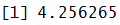
Standard Deviation for dataset Scores_A:

sd(Score_A)

2.726414

Standard Deviation for dataset Scores_B:

sd(Score_B)

4.067486

Standard Deviation for the variable ‘Height.cm.’ in the Height dataset:

sd(HeightData1$Height.cm.)

4.256265

Summary Statistics

One can also use the summary function for summary statistics.

summary(Score_A)

Summary statistics for Scores_A: Min, 1st Qu, Median, Mean, 3rd Qu, Max — Output: summary statistics for Scores_A.

Measures of Shape

In the Theory section of Descriptive Statistics, Measures of Shape were explored in order to see how our dataset is distributed, i.e. whether the distribution is normal or skewed. To find this, we either plot the dataset or calculate the level of skewness or kurtosis.

If our dataset has a bell-shaped curve, then our dataset is normally distributed. Here, the mean, median and mode are equal and all lie in the middle.

We can calculate or visualize skewness which tells us to what degree our data is skewed. If most of the observations lie on the left side of the graph then it is called negatively skewed data, where the mean < median. The vice-versa of this would be called positively skewed data. Kurtosis is based on the height of the curve. A lot of modeling algorithms require the dataset to be normally distributed. Therefore, we use measures of skewness to check for normality. If the dataset is skewed then we transform the variable to normalize the dataset. (This is discussed in detail in the Feature Engineering blog.)

We take the scores data (used above) to measure skewness and kurtosis.

Calculating Skewness

To calculate skewness in R we will first install and load the package e1071. (Type 2 is the sample-adjusted estimator that matches the default skewness method used by Python’s pandas, which is why the values agree.)

install.packages("e1071")
library(e1071)
skewness(Score_A,type = 2)

-0.7327419

Calculating Kurtosis

Here also Type 2 is the excess-kurtosis (Fisher) estimator that matches the default used by Python’s pandas.

library(e1071)
kurtosis(Score_A,type = 2)

-0.325249

Normal Distribution

Visually, anything which doesn’t look like a normal distribution is either skewed or has kurtosis, or is bimodal or multimodal. Therefore it is important to first know how a normally distributed dataset looks like.

Import Dataset: We import a hypothetical dataset having exam scores of students where the mean = mode = median.

Marks_Scored <- read_excel("C:/Users/user/Desktop/Data Sets/Marks_Scored.xls")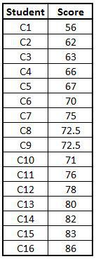

Marks_Scored dataset with Student and Score columns — Output: the exam-scores dataset.

To plot the density we use the command probability equal to TRUE in the histogram. The command lines adds the density curve to the graph while lwd defines the thickness of the line, main is used for the title of the chart.

I <- Marks_Scored$Score
W <- I
hist(W,probability = T,col="blue",xlab="Score",main="Normal Distribution")
lines(density(W),col="green",lwd=2)

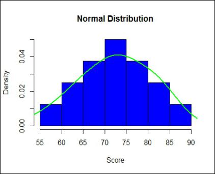
Histogram with density curve of exam scores forming a bell-shaped curve — Output: histogram with density curve of the exam scores.

We can see that the distribution forms a bell-shaped curve which tells us that the dataset is normally distributed. Similarly, we can plot other datasets and if they show similarity to the shapes discussed in the Measures of Shape then they may not be normal.

In this blog, we applied the concepts explored in the theory part of Descriptive Statistics. R is a powerful tool and can be used for univariate and bivariate analysis using various descriptive statistics. It provides tools to perform various statistical calculations along with visualising the dataset. In the next blog, the concepts of Inferential Statistics explored in the Theory section have been put to use using R.