Dimensionality Reduction in Python

There are many modeling techniques that work in the unsupervised setup that can be used to reduce the dimensionality of the dataset. Under the theory section of Dimensionality Reduction, two of such models were explored - Principal Component Analysis and Factor Analysis. In this blog we will use these two methods to see how they can be used to reduce the dimensions of a dataset.

Principal Component Analysis

Here we will explore the most important method of Feature Extraction which is Principal Component Analysis and will use this method to reduce the features and use the output in modeling.

Importing Packages

We first import the important libraries.

import numpy as np
import pandas as pd
import matplotlib.pyplot as plt
%matplotlib inline
from sklearn.decomposition import PCA

Dataset

Here also we will be using the Boston Dataset. We will import a preprocessed dataset. This dataset has also been used in the Regression Problems using Python where the preparation of this dataset has also been explored.

BosData = pd.read_excel('C:/Users/user/Desktop/R - Basic Stats/BosData.xls')
BosData.head()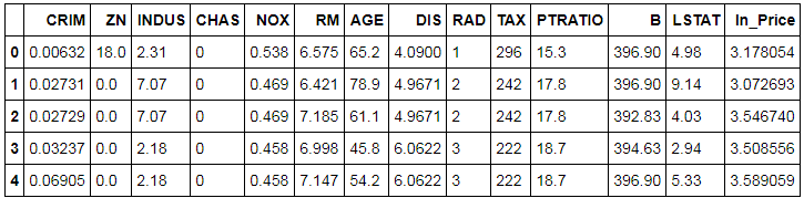

Removing Response Variable

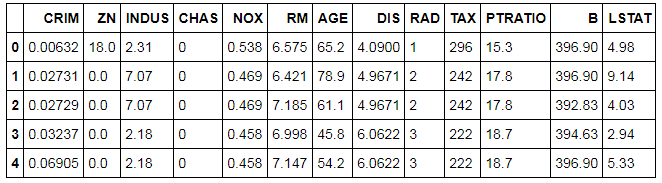
As PCA works in an unsupervised learning setup, therefore we will remove the dependent i.e. response variable from our dataset. Note that PCA only works on numeric variables, and that is why we create dummy variables for categorical variables. As here we have only one categorical variable 'Chas' which is a binary categorical variable, we don't require creating a dummy variable and can use all the independent variables for performing PCA.

BosData2 = BosData[['CRIM', 'ZN', 'INDUS', 'CHAS', 'NOX', 'RM', 'AGE', 'DIS', 'RAD', 'TAX','PTRATIO', 'B', 'LSTAT']]
BosData2.head()

Scaling Features

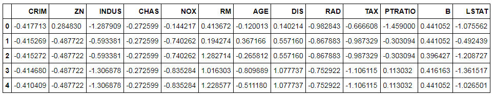
Unlike R, there is no inbuilt option in the PCA command to scale the dataset. Therefore, we will have to first scale the dataset to perform PCA in Python.

from sklearn.preprocessing import StandardScaler
scale = StandardScaler()
scaled_data = scale.fit_transform(BosData2)
scaled_data

We can change the above output into a dataset.

scaled_data = pd.DataFrame(scaled_data,columns=BosData2.columns)
scaled_data.head()

Splitting the Dataset into Train and Test

It is important to note at this point that PCA should not be made to run on the entire dataset as this would cause the dataset to leak thus causing overfitting.

Also, we should not perform PCA on train and test separately as the level of variance will be different in both these datasets which will cause the final vectors of these two datasets to have different directions. This is a Catch-22 situation and to get out of it we first divide the dataset into train and test and perform PCA on the train dataset and transform the test dataset using that PCA model (that was fitted on the train dataset). Below we use the sklearn package to split the data into train and test.

from sklearn.model_selection import train_test_split
Y = BosData['ln_Price']
X_train,X_test,Y_train,Y_test=train_test_split(scaled_data,Y,test_size=0.3,random_state=123)

Initialize and Fit PCA

We first initialize PCA for having 13 components (for 13 continuous variables in the dataset) and then we fit this model on the scaled features.

pca = PCA(n_components=13)
pca_model = pca.fit(X_train)

Generate PCA Loadings

We use the transform command which transforms the scaled data to PCA loadings for each observation.

pca_train = pca_model.transform(X_train)
pca_train

Generate Loading Matrix

We now generate the principal components loading matrix by using the attribute components_ of the pca command for each variable.

Variable_Names =['crim','zn','indus','chas','nox','rm','age','dis','rad','tax','ptratio','black','lstat']
Matrix = pd.DataFrame(pca_model.components_,columns=Variable_Names)
Matrix1 = np.transpose(Matrix)
Matrix1

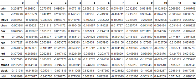
This Loading Matrix is like a correlation matrix. The variable having the highest correlation with the columns will be the first principal component. For example, the variable indus has the highest correlation with PC1, therefore, indus will be PC 1. (The heading in the output is the PC1, PC2 and so on. We will be renaming them in the upcoming steps).

Variance Explained by Each Principal Component

As we saw above, we took the number of components for PCA equal to the number of variables in our dataset (which is 13 in our case). However, now with the following code, we will figure out the optimum value of the number of components to run PCA i.e. reduce the number of components to be considered for the modeling algorithms and thus in a way reducing the number of features. In order to decide the number of Principal Components, we analyze the proportion of variance explained by each component. We use the explained_variance function for computing variance explained by each Principal Component.

pca_model.explained_variance_

Ratio of Variance Explained by Each Component

We can now look at the proportion of variance explained by each PC.

var = pca_model.explained_variance_ratio_
var

From the output we find that PC1 explains 47% of the variance, PC2 explains 11% and so on. We find that the first seven components explain approximately 90% of the variance (0.47818141 + 0.10745023 + 0.09150656 + 0.06383847 + 0.06069613 + 0.0528423 + 0.04414302 = 0.89865812).

PCA Chart

In the above step, we got the proportion of variance explained by each component which we need to decide the number of components. We calculated that the first seven components explain most of the variance, however, for a more visual approach, we plot the explained variance on a line graph. Here we plot the ratio of variance explained by each component using a line graph. This PCA chart helps us to decide the number of principal components to be taken for the modeling algorithm.

cumulative_var = np.cumsum(np.round(var, decimals=4)*100)
plt.plot(cumulative_var,'k-o',markerfacecolor='None',markeredgecolor='k')
plt.title('Principal Component Analysis',fontsize=12)
plt.xlabel("Principal Component",fontsize=12)
plt.ylabel("Cumulative Proportion of Variance Explained",fontsize=12)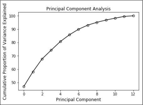

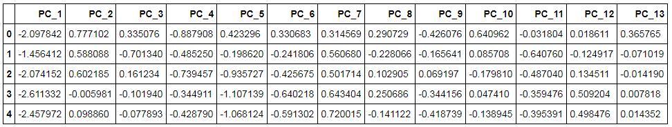
Renaming Columns

For our ease and convenience, we will rename the columns of the loading matrix that was generated for each observation using PCA. After renaming, we will select 7 principal components and make a data frame with the dependent variable and the 7 PCs.

pca_train = pd.DataFrame(pca_train,columns=['PC_' + str(i) for i in range(1, 14)])
pca_train.head()

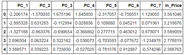
Concatenate Dependent Variable and Principal Components

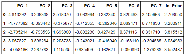
We now concatenate the dependent variable i.e. ln_Price with principal components and take the first seven components for our analysis. First, we will reset the index for Y_train as we need to concatenate datasets to make one whole train dataset. Then we will remove the index variable from the dataset and make a subset of the dataset having 7 PCs and the dependent variable.

Y_train1 = Y_train.reset_index()

pca_train1 = pd.concat([pca_train,Y_train1],axis=1)
pca_train2 = pca_train1.drop(columns='index')
pca_train3 = pca_train1[['PC_1', 'PC_2', 'PC_3', 'PC_4', 'PC_5', 'PC_6', 'PC_7','ln_Price']]

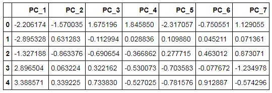
Creating Dataset Having Principal Components

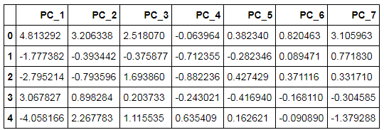
The above output forms the complete train dataset. As now we will be performing linear regression on this dataset we are required to create a separate dataset having all the principal components i.e. the independent features.

pca_train_X = pca_train3[['PC_1', 'PC_2', 'PC_3', 'PC_4', 'PC_5', 'PC_6', 'PC_7']]
pca_train_X.head()

Initializing and Fitting Linear Regression Model

We use linear_model from sklearn and initialise a Linear Regression Model.

from sklearn import linear_model
linreg_model = linear_model.LinearRegression()
linreg_model.fit(pca_train_X,Y_train)

Transform Features of Test Dataset into Principal Components

As mentioned earlier, we will transform the features of the dataset into Principal Components using the PCA model created earlier.

pca_test = pca.transform(X_test)
pca_test

We now convert the above output into a dataset and add the dependent variable to it so that we can predict values using the above created linear regression.

pca_test = pd.DataFrame(pca_test,columns=['PC_' + str(i) for i in range(1, 14)])
Y_test1 = Y_test.reset_index()
pca_test1 = pd.concat([pca_test,Y_test1],axis=1)
pca_test1 = pca_test1.drop(columns='index')
pca_test2 = pca_test1[['PC_1', 'PC_2', 'PC_3', 'PC_4', 'PC_5', 'PC_6', 'PC_7','ln_Price']]
pca_test2.head()

Above we got the complete dataset. We now separate the Principal Components in a separate dataset.

pca_test_X = pca_test2[['PC_1', 'PC_2', 'PC_3', 'PC_4', 'PC_5', 'PC_6', 'PC_7']]
pca_test_X.head()

Prediction

We now predict the dependent variable of the test dataset using the linear regression model created earlier.

predict1 = linreg_model.predict(pca_test_X)

Results

We calculate the R-square to know the accuracy of our model.

from sklearn import metrics
metrics.r2_score(Y_test,predict1)

The accuracy comes out to be 63%.

Factor Analysis

Factor Analysis is a method which works in an unsupervised setup and forms groups of features by computing the relationship between the features. It is commonly used to reduce features and is explored in Factor Analysis under the theory section. We will now explore the application of Factor Analysis in Python. Factor analysis can only be used to reduce continuous variables of the dataset. Therefore, we will be removing categorical variables. Again, like principal component analysis, this is an unsupervised learning algorithm and hence we will be removing the dependent variable from our dataset.

Importing Preliminary Libraries

From factor_analyzer we will import FactorAnalyzer which will come handy for performing factor analysis.

from factor_analyzer import FactorAnalyzer

Dataset

We will be using the pre-processed Boston dataset that we have already normalized by creating a new variable ln_Price which is log of the dependent variable i.e. Price.

Bos_train2 = pd.read_excel('C:/Users/user/Desktop/Data Sets/Linear Regression/Bos_train1.xls')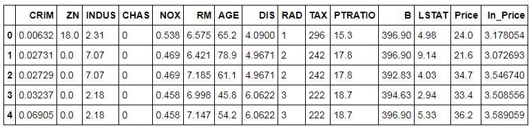

Removing the Dependent and Categorical Variables

As mentioned above, factor analysis works in an unsupervised setup only for the numerical variables, therefore, we will get rid of the categorical and the dependent variable.

Factor1 =Bos_train2[['CRIM', 'ZN', 'INDUS','NOX', 'RM', 'AGE', 'DIS', 'RAD', 'TAX','PTRATIO', 'B', 'LSTAT']]

Creating Correlation Matrix for the Above Dataset

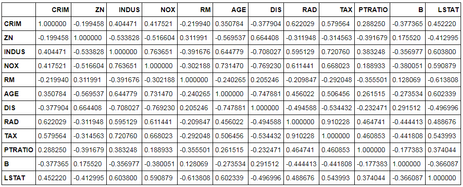
To perform factor analysis we first create a correlation matrix using the above dataset. We can also manually analyse this matrix as this will give us an idea of the variables that are highly correlated with each other.

corrm = Factor1.corr()
corrm

Show full table ▾

Finding Eigen Values

We will now find the eigenvalues to decide the number of factors that will be sufficient for our modeling i.e. deciding the number of variables we will use during modeling.

eigen_values = np.linalg.eigvals(corrm)
eigen_values_cumvar = (eigen_values/12).cumsum()
eigen_values_cumvar

Clearly, the four factors explain approximately 79% of the variance. Therefore, the number of factors will be equal to 4 in our case.

Using Factor Analyzer to Perform Factor Analysis

Now we will compute the factor loadings to group the variables based on their correlation values.

Factor_Analysis = FactorAnalyzer(n_factors=4, rotation='varimax', method='ml')
Factor_Analysis.fit(Factor1)

Here, we have used rotation equal to varimax to get maximum variance and the method deployed for factor analysis is maximum likelihood. R and Python use methods - maximum likelihood or minres. However other software such as SAS uses the method principal component analysis (PCA) to compute factor loadings.

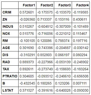
Compute Factor Loadings

We now compute factor loadings.

loadings = pd.DataFrame(Factor_Analysis.loadings_, index=Factor1.columns)
loadings

We now export the above output and sort it to find the 4 groups of features.

loadings.to_excel('C:/Users/user/Desktop/Data Sets/Linear Regression/python_FA.xls')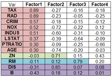

We can select variables for each of these groups which will help us in decreasing the features and decrease the chances of multicollinearity.

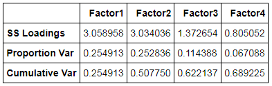
We can also compute the proportional variance and cumulative variance of the 4-factor solution.

Factor_Analysis.get_factor_variance()

There are many more algorithms such as decision trees which work in a supervised setup and can be used to reduce the dimensionality of the dataset. In unsupervised setup, PCA and factor analysis are the most commonly used models to reduce the dimensionality of the dataset. Both these methods have been put to use for reducing the dimensionality of the dataset using R in the blog Dimensionality Reduction in R.