// application · python

Clustering Problems in Python

Clustering Problems are one of the most common problems solved in an Unsupervised Environment. Various clustering algorithms provide us with a method of grouping observation in such a way that the observations in the same group are similar to each other than those in other groups. As mentioned above, this is an unsupervised modeling technique, as here we do not control how the clusters will be made. The only thing that we can control in this modeling is the number of clusters and the method deployed for clustering. Various clustering techniques have been explained under Clustering Problem in the Theory Section. In this blog, we will explore three clustering techniques using python: K-means, DBScan, Hierarchical Clustering.

Preparation

Adding Preliminary Libraries

We first add some important libraries that will be useful for us throughout the course.

import numpy as np
import pandas as pd
import matplotlib.pyplot as plt
%matplotlib inline

Importing Dataset

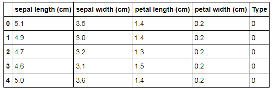
To demonstrate various clustering algorithms in python, the Iris dataset will be used which has three classes in the dependent variable (three type of Iris flowers) and using this dataset clusters will be formed.

from sklearn import datasets
iris = datasets.load_iris()
iris_data = pd.DataFrame(iris.data)
iris_data.columns = iris.feature_names
iris_data['Type']=iris.target
iris_data.head()

Show full table ▾

Preparing Data

Here we have the target variable 'Type'. We need to remove the target variable so that this dataset can be used to work in an unsupervised learning environment. The iloc function is used to get the features we require. We also use .values function to get an array of the dataset. (Note that we transformed the dataset to an array so that we can plot the graphs of the clusters).

iris_X = iris_data.iloc[:, [0, 1, 2,3]].values

Now we will separate the target variable from the original dataset and again convert it to an array by using numpy.

iris_Y = iris_data['Type']
iris_Y = np.array(iris_Y)

Visualise Classes

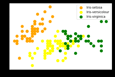
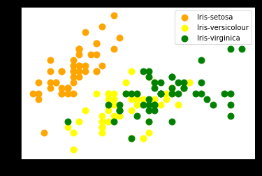
In this Iris dataset, we have three classes. We visualise these classes in a 2-D graph. This will help us in comparing the original classes with the clusters created by the different clustering algorithms. We use the following code to plot the original dataset visualise the three type of flowers on a graph.

plt.scatter(iris_X[iris_Y == 0, 0], iris_X[iris_Y == 0, 1], s = 80, c = 'orange', label = 'Iris-setosa')
plt.scatter(iris_X[iris_Y == 1, 0], iris_X[iris_Y == 1, 1], s = 80, c = 'yellow', label = 'Iris-versicolour')
plt.scatter(iris_X[iris_Y == 2, 0], iris_X[iris_Y == 2, 1], s = 80, c = 'green', label = 'Iris-virginica')
plt.legend()

We find that we have three classes with two types of Iris flowers overlapping each other.

Clustering Algorithms

In this blog, we will be discussing three main ways to create clusters out of the Iris dataset, which are

• K-Means
• DBSCAN
• Agglomerative Clustering aka Hierarchical Clustering

K-Means Clustering

One of the most commonly used methods of clustering is K-means Clustering which allows us to define the required number of clusters. To know about the workings of K-means refer to the blog: K-Means in the Theory Section.

Importing Library

We import KMeans from sklearn.cluster to run a K-Means model.

from sklearn.cluster import KMeans

Deciding Value of K

The most crucial aspect of K-Means clustering is deciding the value of K. We do this by performing elbow analysis. Refer to the K-Means Theory blog for more information on why and how this actually works. We first run Kmeans for the value of K from 1 to 11.

wcss = []
for i in range(1, 11):
    kmeans = KMeans(n_clusters = i, init = 'k-means++', max_iter = 300, n_init = 10, random_state = 0)
    kmeans.fit(iris_X)
    wcss.append(kmeans.inertia_)

We now plot the WCSS obtained from the above code. WCSS or within-cluster sum of squares is a measure of how internally coherent the clusters are. K-Means tries to minimize this criterion.

plt.plot(range(1, 11), wcss)
plt.title('The elbow method')
plt.xlabel('Number of clusters')
plt.ylabel('WCSS')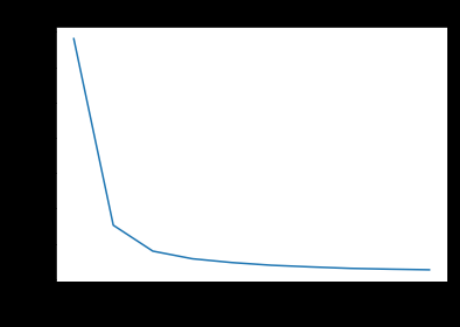

In the elbow graph, we look for the points where the drop falls and the line smoothens out. In the above graph, this happens for k=3. Another way of understanding this is that we note the point at which the WCSS is less and try to find the number of clusters for our dataset. We see that at the number of clusters = 3, WCSS is less than 100, which is good for us. So we take k =3.

Running K-Means Model

We now run K-Means clustering for obtaining a 3 cluster solution.

cluster_Kmeans = KMeans(n_clusters=3)
model_kmeans = cluster_Kmeans.fit(iris_X)
pred_kmeans = model_kmeans.labels_
pred_kmeans

Visualizing Output

In the above output we got value labels: '0', '1' and '2'. For a better understanding, we can visualize these clusters.

plt.scatter(iris_X[pred_kmeans == 0, 0], iris_X[pred_kmeans == 0, 1], s = 80, c = 'orange', label = 'Iris-setosa')
plt.scatter(iris_X[pred_kmeans == 1, 0], iris_X[pred_kmeans == 1, 1], s = 80, c = 'yellow', label = 'Iris-versicolour')
plt.scatter(iris_X[pred_kmeans == 2, 0], iris_X[pred_kmeans == 2, 1], s = 80, c = 'green', label = 'Iris-virginica')
plt.legend()

When compared to the original classes we find that the observations of the class label Iris-setosa has been correctly formed into a separate well-defined cluster, however, for the other two classes, clusters are not as correct. This is mainly because, in the original dataset, these two class labels were overlapping each other which makes it difficult for the clustering algorithm as it works best for clear neat separate observations. Still, the clusters have been formed. more or less correctly.

DBScan

DBScan, an acronym for Density-Based Spatial Clustering of Applications with Noise is a clustering algorithm. It makes clusters based on their densities. It identifies observations in the low-density region as outliers.

Importing Library

We import DBSCAN from sklearn.cluster to run a DBScan model.

from sklearn.cluster import DBSCAN
clt_DB = DBSCAN()

Initialize Model

We now initialise the DBScan Model with eps (epsilon) = 0.42

clt_DB = DBSCAN(eps=0.42)
clt_DB

Fit Model

In this step, we fit the model on the iris dataset and come up with the class labels.

model_dbscan = clt_DB.fit(iris_X)
pred_dbscan = model_dbscan.labels_
pred_dbscan

Visualizing Output

In the above output, we got value labels: '0', '1', '2' and '-1' with the '-1' label indicting outliers. We visualise this output to see how the data has been grouped into clusters.

plt.scatter(iris_X[pred_dbscan == 0, 0], iris_X[pred_dbscan == 0, 1], s = 80, c = 'orange', label = 'Iris-setosa')
plt.scatter(iris_X[pred_dbscan == 1, 0], iris_X[pred_dbscan == 1, 1], s = 80, c = 'yellow', label = 'Iris-versicolour')
plt.scatter(iris_X[pred_dbscan == 2, 0], iris_X[pred_dbscan == 2, 1], s = 80, c = 'green', label = 'Iris-virginica')
plt.scatter(iris_X[pred_dbscan == -1, 0], iris_X[pred_dbscan == -1, 1], s = 80, c = 'red', label = 'outlier')
plt.legend()

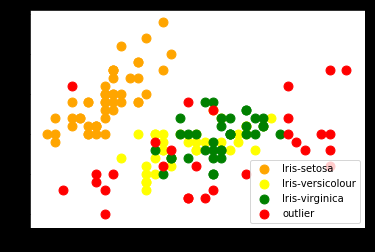
We find that by using DB Scan some observations are marked as outliers.

Hierarchical Clustering

Hierarchical Clustering can be of two types- Agglomerative and Divisive. In this blog post, we will explore Agglomerative Clustering which is a method of clustering which builds a hierarchy of clusters by merging together small clusters. To know more about Hierarchical Clustering refer to the blog Hierarchical Clustering under the Theory Section.

Import Library

We first import the package AgglomerativeClustering using which we will create an agglomerative clustering model.

from sklearn.cluster import AgglomerativeClustering

Plotting of Dendrogram

We make use of dendrogram to decide the number of clusters required for our dataset. A dendrogram is a tree diagram which illustrates the arrangement of clusters.

We first start off by importing the library that will allow us to create dendrograms.

import scipy.cluster.hierarchy as sch

We now pick the features from the original dataset.

iris_X = iris_data[['sepal length (cm)','sepal width (cm)','petal length (cm)','petal width (cm)']]

We finally plot a Dendrogram which allows us to see what the threshold values should be for the clustering algorithm. Basically, we decide the number of clusters by using this dendrogram.

Z = sch.linkage(iris_X, method = 'median')
plt.figure(figsize=(20,7))
den = sch.dendrogram(Z)
plt.title('Dendrogram for the clustering of the dataset iris')
plt.xlabel('Type')
plt.ylabel('Euclidean distance in the space with other variables')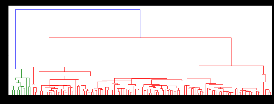

Building an Agglomerative Clustering Model

Initialise Model

We analyse the above-created dendrogram and decide that we will be making 3 clusters for this dataset.

cluster_H = AgglomerativeClustering(n_clusters=3)

Fitting Model

After building Agglomerative clustering, we will fit our iris data set. (Note that only the independent variables from the Iris dataset are taken into account for the purpose of clustering.)

model_clt = cluster_H.fit(iris_X)
model_clt

We now come up with the class labels.

pred1 = model_clt.labels_
pred1

Visualizing Output

We use the above-found class labels and visualise how the clusters have been formed.

plt.scatter(iris_X.values[pred1 == 0, 0], iris_X.values[pred1 == 0, 1], s = 80, c = 'orange', label = 'Iris-setosa')
plt.scatter(iris_X.values[pred1 == 1, 0], iris_X.values[pred1 == 1, 1], s = 80, c = 'yellow', label = 'Iris-versicolour')
plt.scatter(iris_X.values[pred1 == 2, 0], iris_X.values[pred1 == 2, 1], s = 80, c = 'green', label = 'Iris-virginica')
plt.legend()

Here also we found that Iris-setosa has been clearly formed into separate cluster while the other clusters overlap each other.

In this blog post, we explored the application of three different clustering algorithms in python. All these algorithms have their own style of functioning and should be used when trying to solve clustering problems. To find the application of these algorithms in R refer to the blog- Clustering Problems in R.