// application · r

Miscellaneous Methods in R

Before we perform modeling on our datasets, we need to prepare the dataset first. This pre-processing of data includes various steps which were explored in Miscellaneous Methods under the section Data Exploration and Preparation. In this blog, we will explore the application of various data preparation methods in R. These methods include the following:

Consolidation of Data Sets
Missing Value Treatment
Outlier Treatment

Note that uni-variate and bi-variate analysis, which are methods of data exploration (and were discussed in the theory section under Data Exploration and Preparation), have already been discussed in the blogs related to the application of descriptive and inferential statistics, as these methods of analysis use various descriptive and inferential statistics.

Consolidation of Data Sets

There are mainly two ways of consolidating datasets: appending and merging.

Appending

Appending of datasets is concatenating or stacking datasets either row-wise or column-wise (whereas merging of datasets is combining datasets based on a common variable).

Import Dataset: Here we have taken two datasets of cars sold by a dealer. (Please note that all datasets used in the sections of coding are hypothetical. If any dataset has been taken from an outside source, the link of the source will be mentioned for that particular dataset.) Note that the variable names should be the same while appending datasets.

We begin with importing the first car dataset.

CarData1 <- read_excel("C:/Users/user/Desktop/Data Sets/Car_Data1.xls")
View(CarData1)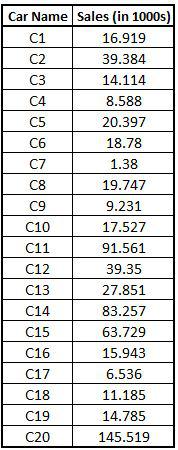

CarData1 dataset with Car Name and Sales in 1000s columns — Output: the CarData1 dataset.

We then upload the second car dataset.

CarData2 <- read_excel("C:/Users/user/Desktop/Data Sets/Car_Data2.xls")
View(CarData2)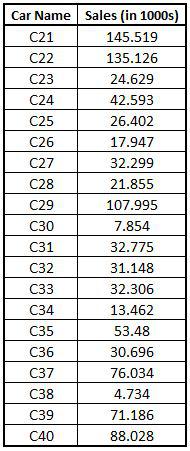

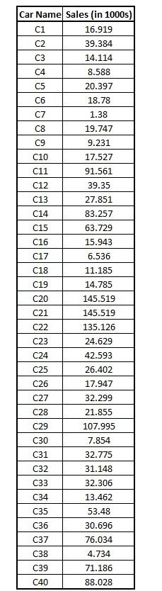
CarData2 dataset with Car Name and Sales in 1000s columns — Output: the CarData2 dataset.

Appending Datasets Row-wise

Here we Append datasets by concatenating the two datasets row-wise. We use the following command to append the two datasets - CarData1 and CarData2. Here the rbind command stacks one dataset under another. It is basically concatenating datasets row-wise.

append1 <- rbind(CarData1,CarData2)
View(append1)

append1 dataset, CarData1 and CarData2 stacked row-wise — Output: append1.

Appending Datasets Column-wise

Here we Append datasets by concatenating the two datasets column-wise. We concatenate the two datasets column-wise. Here we use the function cbind.

col_concat <- cbind(CarData1,CarData2)

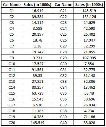
col_concat dataset, CarData1 and CarData2 joined column-wise — Output: col_concat.

Renaming Columns: We rename the columns so as to easily differentiate between the two datasets.

colnames(col_concat) <- c('Car_Name1','Sales in 1000s','Car_Name2','Sales in 1000s')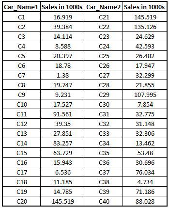

col_concat dataset with renamed columns — Output: col_concat with renamed columns.

Merging

Merging of datasets is mainly used to combine datasets with common values. We use joins to merge datasets based on our requirement. First, we will do the normal merging of datasets. This is equivalent to appending of datasets column-wise. In merging, at least one variable has to be common in both datasets, on the basis of which merging will take place.

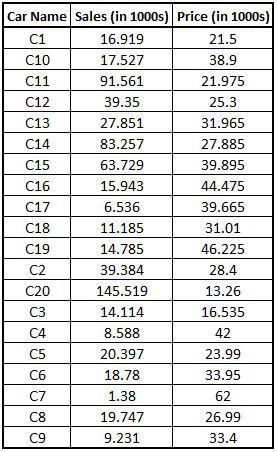
Importing Dataset: We import a dataset where, unlike CarData1 and CarData2 (where we had the sales information of the car), here we will have a Price variable.

CarData3 <- read_excel("C:/Users/user/Desktop/Data Sets/Car_Data3.xls")

Simple Merge: We use the merge function. The following command is equivalent to appending the data column-wise.

Merged1 <- merge(CarData1,CarData3,by="Car Name")
View(Merged1)

Merged1 dataset, CarData1 merged with CarData3 on Car Name — Output: Merged1.

Ways of Joining Tables

As mentioned in Consolidation of Datasets, there are various ways of joining two datasets and we will be exploring some of them here.

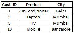
Import Datasets: In order to explain different joins, we will be using two datasets of a store. One has information of the product bought by the customer and the other dataset has the city of residence of that customer.

Importing the first Store dataset.

StoreData1 <- read_excel("C:/Users/user/Desktop/Data Sets/Store_Data1.xls")
View(StoreData1)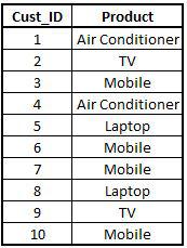

StoreData1 dataset with Cust_ID and Product columns — Output: the StoreData1 dataset.

Importing the second Store dataset.

StoreData2 <- read_excel("C:/Users/user/Desktop/Data Sets/Store_Data2.xls")
View(StoreData2)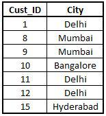

StoreData2 dataset with Cust_ID and City columns — Output: the StoreData2 dataset.

We can now perform the various methods of merging these two datasets. In this blog, we will perform Inner Join, Outer Join, Left Join and Right Join.

Inner Join

An inner join is used to find the common information between the two datasets, i.e. it is the intersection of two datasets. Here it takes the common entries of the customers from both the datasets and makes a table with their corresponding entries. Note - the function merge by default takes inner join. You can specify the type of join by using the command all in the merge function.

Inner1 <- merge(x=StoreData1,y=StoreData2,by.x = "Cust_ID")
View(Inner1)

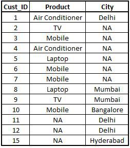
Inner1 dataset, the inner join of StoreData1 and StoreData2 — Output: Inner1.

Outer Join

Outer Join takes all the entries of both the datasets even if the entry for a variable is missing for that customer in either of the datasets. Basically, it is the union of both the datasets. In the outer join, we mention all = T (True) to specify we want to merge both datasets completely.

Outer1 <- merge(x=StoreData1,y=StoreData2,by="Cust_ID",all=T)
View(Outer1)

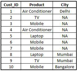
Outer1 dataset, the outer join of StoreData1 and StoreData2 — Output: Outer1.

Left Join

Left join gives you the details of customers in dataset 1 and their corresponding entries from dataset 2. It does not take any entry of the customer that is present in dataset 2 and not in dataset 1. In left join, we mention all.x=T, i.e. take all information of the left dataset which is x.

Left1 <- merge(x=StoreData1,y=StoreData2,by="Cust_ID",all.x=T)
View(Left1)

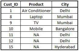
Left1 dataset, the left join of StoreData1 and StoreData2 — Output: Left1.

Right Join

Right Join is similar to the left join. While the Right Join takes all entries of dataset 2 and corresponding entries of dataset 1. In the left join, it's the other way around. Here we take all.y = T (True), i.e. take all information from the right dataset, i.e. y.

Right1 <- merge(x=StoreData1,y=StoreData2,by="Cust_ID",all.y =T)
View(Right1)

Right1 dataset, the right join of StoreData1 and StoreData2 — Output: Right1.

Missing Value Treatment

The next main step of data preparation is missing value treatment. The data at hand may or may not have missing values. But if the dataset has missing values, then we will have to treat them first, either by removing them or replacing them with the mean, median or mode, depending on the type of the variable.

Import Dataset: We use a car sales dataset having multiple variables and perform missing value treatment on it.

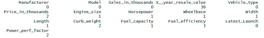
carsales <- read.csv("C:/Users/user/Desktop/Data Sets/car_sales.csv")

Checking Missing Values: Before treating the missing values, we need to check if the data has missing values or not. In order to check for the missing values, we use the sapply function in R. Here we count the missing values and take a sum of them so that for each variable we know the number of missing values present in them.

sapply(carsales, function(x) sum(is.na(x)))

Missing value counts per column of the carsales dataset — Output: count of missing values per variable.

Methods of Treating Missing Values

Now the missing values can be either in the continuous or categorical variables. There are mainly two methods to deal with missing values, which are discussed below.

Remove the missing values: Here we use the na.omit command to drop the observations where we have missing values. As discussed in Missing Value Treatment (under the Theory section), this method causes loss of valuable data. However, sometimes the datasets have very few missing values, therefore we can remove those observations by using this method.

carsalesNew <- na.omit(carsales)

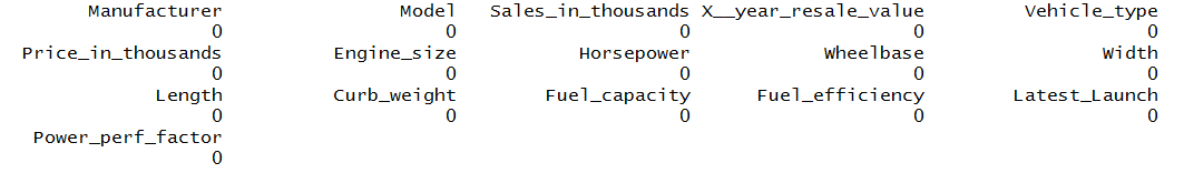
We can now again use the sapply function to see if there are any missing values in the dataset or not.

sapply(carsalesNew, function(x) sum(is.na(x)))

Missing value counts per column after na.omit, all zero — Output: count of missing values after removal - all zero.

Mean, Median and Mode Imputation: In this method, we impute the missing values with the mean, median or mode of their respective variable.

Mean Imputation

We impute the missing values with the mean of their variable.

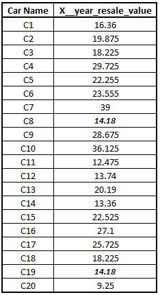
Import Dataset: We import a dataset having missing values in a continuous variable.

CAR1 <- read_excel("C:/Users/user/Desktop/Data Sets/CAR1.xls")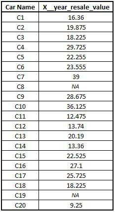

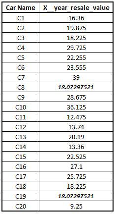
CAR1 dataset with Car Name and X__year_resale_value columns, including missing values — Output: the CAR1 dataset.

Performing Mean Imputation: We now perform mean imputation using the is.na function and replace the missing values with the mean. na.rm is set to TRUE to tell the program to ignore the NAs while calculating the mean.

CAR1$X__year_resale_value[is.na(CAR1$X__year_resale_value)]<-
mean((CAR1$X__year_resale_value),na.rm=T)
View(CAR1)

CAR1 dataset after mean imputation, missing values replaced by 18.07297521 — Output: CAR1 after mean imputation.

Median Imputation

We impute the missing values with the median value of their variable.

Import Dataset: We import a dataset having missing values in a continuous variable.

CAR2 <- read_excel("C:/Users/user/Desktop/Data Sets/CAR1.xls")

Performing Median Imputation: We perform median imputation using the same function as we did for mean imputation. Only the mean gets replaced by the median.

CAR2$X__year_resale_value[is.na(CAR2$X__year_resale_value)]<-
median((CAR2$X__year_resale_value),na.rm=T)
View(CAR2)

CAR1 dataset after median imputation, missing values replaced by 14.18 — Output: CAR2 after median imputation.

Mode Imputation

We impute the missing values of a categorical variable with its mode.

Import Dataset: We import a dataset having missing values in a categorical variable.

CAR3 <- read_excel("C:/Users/user/Desktop/Data Sets/CarTypeData.xls")
View(CAR3)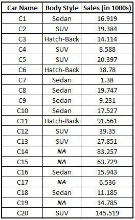

CAR3 dataset with Car Name, Body Style and Sales in 1000s columns, including missing Body Style values — Output: the CAR3 dataset.

Creating Function: R does not have an in-built function for mode. Therefore, we will create a function to compute mode and it will be saved in the global environment for future use. Run the following code in the editor window.

getmode <- function(v) {
  uniqv <- unique(v)
  uniqv[which.max(tabulate(match(v,uniqv)))]
}

Now we will use the above function to compute the mode for the dataset.

v <- CAR3$`Body Style`
mode <- getmode(v)
mode

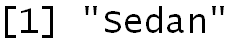
Mode output, Sedan — Output: the mode of Body Style is "Sedan".

We find that the mode comes out to be 'Sedan', which means that we should replace all the missing values of the 'Body Style' variable with 'Sedan'.

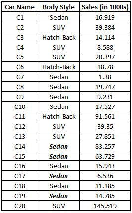
Performing Mode Imputation: We now perform Mode Imputation on the Car dataset.

CAR3$`Body Style`[is.na(CAR3$`Body Style`)] <- mode

CAR3 dataset after mode imputation, missing Body Style values replaced by Sedan — Output: CAR3 after mode imputation.

KNN Imputation

There is also an unsupervised method for imputing missing values in a dataset, called KNN imputation. It uses the K-Nearest Neighbours algorithm to impute the missing values of categorical and continuous variables.

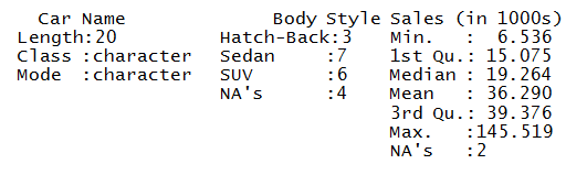
Let us import the dataset with missing values in both categorical and continuous variables.

Data7 <- read_excel("C:/Users/user/Desktop/Data Sets/MissingData.xls")

We will first convert the variable Body Style to factor using the following code.

Data7[,'Body Style'] <- lapply(Data7[,'Body Style'],factor)
summary(Data7)

Summary of Data7 showing Body Style factor levels and Sales statistics with NAs — Output: summary of Data7.

Importing the library VIM.

library(VIM)

We specify the variables which have missing values, irrespective of the type of the variable.

New1 <- kNN(Data7,variable = c("Body Style","Sales (in 1000s)"))
New2 <- New1[1:3]
summary(New2)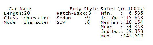

Summary of New2 after KNN imputation, no NAs remaining — Output: summary after KNN imputation.

There are other sophisticated methods, such as using Linear and Logistic Models, to predict the missing values and replace the missing values with them. All such models have been discussed in the Application part of the Modeling section.

Outlier Treatment

Apart from Missing Value Treatment, the other most important and crucial preprocessing/data preparation step is Outlier Treatment. We have found under the Application of Basic Statistics how outliers can affect the dataset, therefore it is very important to do outlier treatment.

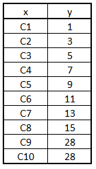
Import Dataset: We import a dataset that contains an outlier.

Outlier <- read_excel("C:/Users/user/Desktop/Data Sets/Outlier 1.xls")
View(Outlier)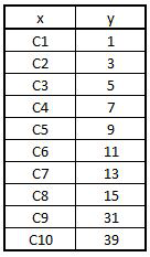

Outlier dataset with x and y columns — Output: the Outlier dataset.

Method of Treating Outliers: In order to do outlier treatment, we calculate a benchmark which will replace the outliers. For this, we take the help of the following:

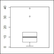
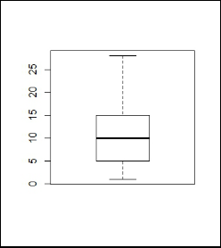
Boxplot

We can create boxplots and identify the outliers. We can also use them to decide the value at which we might want to cap the outliers.

boxplot(Outlier$y)

Boxplot of y showing two outlier points above 30 — Output: boxplot of y before treatment.

Quartiles

We can use the quartiles method to calculate the benchmark and replace the outliers with that benchmark.

summary(Outlier$y)

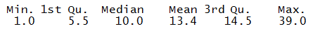
Five-number summary of Outlier y: Min 1.0, 1st Qu 5.5, Median 10.0, Mean 13.4, 3rd Qu 14.5, Max 39.0 — Output: summary statistics of Outlier$y.

We use the above statistics for further calculations.

bench <- 14.5 + 1.5*IQR(Outlier$y)
bench

[1] 28

Unlike Python, we don't have to calculate the IQR (Inter-Quartile Range) manually - R's IQR() function does it directly.

Outlier$y[Outlier$y > bench] <- bench

Outlier dataset after capping, the two values above 28 replaced with 28 — Output: the Outlier dataset after capping.

Creating a boxplot to check visually if there are any outliers in the dataset or not.

boxplot(Outlier$y)

Boxplot of y after capping, no outlier points remain — Output: boxplot of y after treatment.

There are various "miscellaneous" methods that come under preprocessing of data or data preparation. In this blog, we explored various such methods. Missing Value and Outlier Treatment act as the most important steps towards making the data clean and usable for various modeling algorithms. Various methods of consolidating datasets were also explored here, which are highly useful to make the analysis more meaningful. Data Preprocessing requires Feature Engineering, and there are multiple methods of performing feature engineering; the application (in R) of all such methods has been explored in the next blog.