// f tests

Repeated Measures ANOVA

In this article, a very intuitive idea about how Repeated Measures ANOVA works is provided and unlike the article on One Way ANOVA, the formula and its calculations will not be explored in full detail.

Repeated Measures ANOVA v/s One Way / Factorial ANOVA

Repeated Measures ANOVA is very similar to Paired T-Test or the One-Way ANOVA. Like One-Way ANOVA where we separated the variance found in the independent variable into variance found between groups and variance found within groups, in Repeated Measures ANOVA we also divide the variance of our dependent variable. However, there are a number of advantages that Repeated Measures ANOVA has over them such as-

Repeated Measures ANOVA tests related groups and is called so because we examine the difference of mean on the dependent variable over more than two time points. Thus for example, if we have a group of students who give a maths exam at the beginning of the year, the same exam in the middle of the year and then again at the end of the year. In this example, the independent variable will be the month (essentially it is time) and the dependent variable is the score of the students.

By using Repeated Measures ANOVA we can control the effects of covariates (covariates are explained in the previous article on Factorial ANOVA, and for now covariates can be understood as simply the variable(s) that are used to control or account for a portion of variance in the dependent variable so we can see the variance explained by an independent variable without being influenced by a covariate, e.g. children play more outside in the USA than they do in Norway, Sweden and the UK, but here the covariate can be the factor of weather and after controlling the variance explained by weather, we see if now the country the children belong to can explain the variance in the playing time). In Repeated Measures ANOVA we can control the effects of more than one covariate (thus can conduct an ANCOVA- Analysis of Covariance).

Like Factorial ANOVA we can have more than one categorical independent variable.

Examples

To explain how Repeated Measures works and the situations where it can be applied, a couple of examples will be used that will give some understanding of the scenarios under which Repeated Measures ANOVA is useful.

First things first, we must remember that Repeated Measures ANOVA is conducted when the data belongs to the same set of participants, however they are collected over different periods of time, and we are to see if the changes are relevant or not. Also, remember that for Repeated Measures ANOVA, the dependent variable should be numeric (continuous) while the independent variable should be categorical.

(The below-mentioned examples are based on the book Statistics in Plain English written by Timothy C. Urdan and contain excerpts from it.)

Example 1

You decide to conduct an experiment where you want to test if consumption of alcohol affects the reaction time in adults when they are driving. We take a group of 50 adults and note the time taken by them to hit the brakes of the car when they are instructed to do so. The reaction time of the same group is taken again after they have consumed 2 more drinks. We have with us now a group with two scores on one dependent variable and here the dependent variable is the reaction time. Now if we ask our participants to consume 2 more drinks we will end up having 3 measures of reaction- first when they were sober, second when they had consumed 2 drinks and third when they had consumed 2 more drinks (by now 4 drinks in total).

Now we use Repeated Measures ANOVA to see the change of mean across the three trials and find that the mean changes over time and is statistically significantly higher, making us conclude that drinks do cause the reaction time to increase. However, the alcohol manufacturer objects to it by saying that our test is flawed as alcohol affects those who weigh less more and we have not considered the weight of our participants, so we decide to include weight as a covariate to partial out the variance explained by weight in the change of reaction time. However, after controlling for the effects of weight, the result stood out to be the same (weight was thus not able to explain any variance in the reaction time of people over time).

Now the alcohol manufacturers come up with a claim that reaction time is also dependent on gender and alcohol slows down the reaction time of “lightweight” females but doesn’t affect “heavier” males. To test this we take a sample where there are 100 males and 100 females who vary in their weights and again test their reaction time while driving after zero, two, and four alcoholic drinks.

“Now I’ve got one dependent variable (reaction time) measured at three time points, one covariate (weight), and one independent group variable (gender of participant). Notice that although the number of drinks is technically an independent variable, it is not a categorical, or group, variable. In other words, I do not have three independent groups (the zero-drink group, the two-drink group, and the four-drink group). Rather, I have three dependent, or repeated, measures of the same dependent variable, reaction time.”

Now after controlling the effect of the covariates, no difference was found in the reaction time, and also no interaction was found between gender and the number of drinks on reaction time. Thus reaction time got slower for both males and females.

Example 2

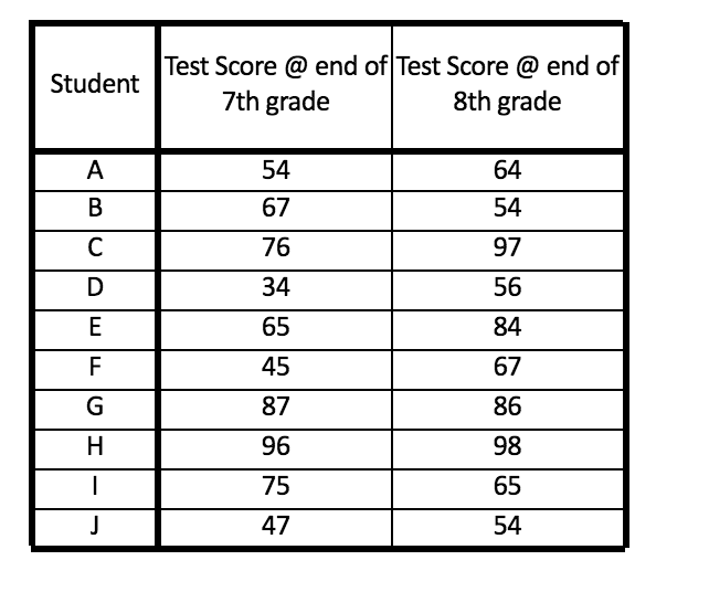
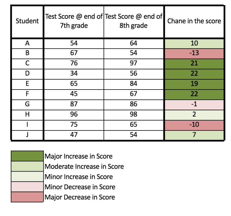
We want to know whether there is an increase in the knowledge of students from one academic year to another. Here time is the change in the academic year. To find if there is a change in the knowledge, a special Aptitude Test is prepared and students are tested on it at the end of the seventh and eighth academic year. The number of students in the group is 10 and in the end, we will have two sets of scores and 20 scores in total. Now we find the average and variance of these scores.

We will use the Repeated Measures ANOVA and will find the sources of these variations, and for this, we partition the total variance into different pieces.

First Source of Variation

The first source of variation in the marks can be the portion of variance attributed to the deviations between the individual scores of the students. For each student, there are two scores and we find the average of their score and compare it with the average of the overall score of all the students, which is 68.55. Example for student A, the average score is 59 (54 + 64 ÷ 2) and this score is compared with the overall average for all the scores.

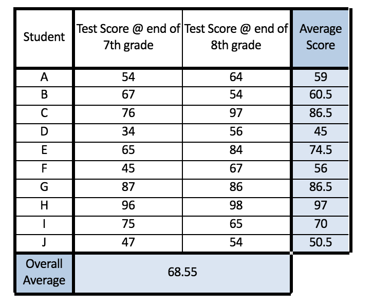
Thus we can see that there is some variation in the average scores of the 10 students and this creates the first source of variation.

Second Source of Variation

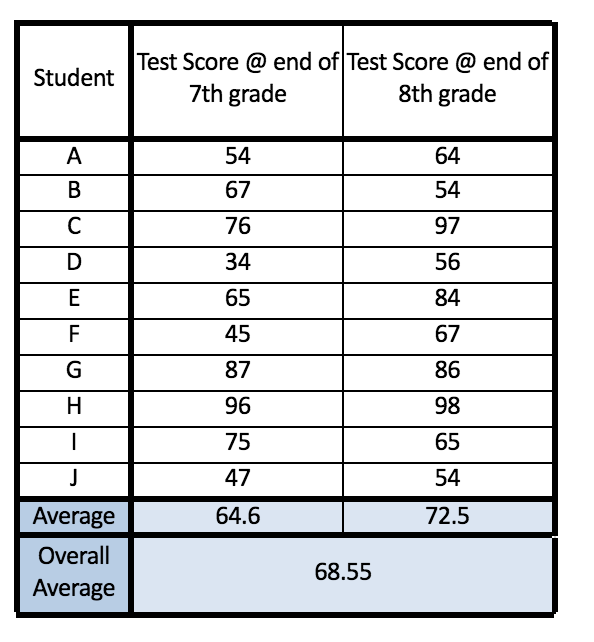
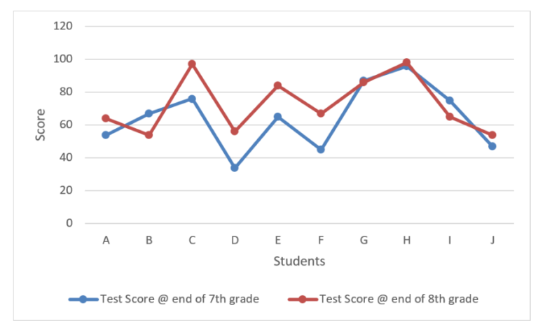
The second source of variation involves the differences in the marks of students from Time 1 (at end of 7th grade) to Time 2 (at end of 8th grade). These changes in the scores of the students are known as the within-subject effects. We calculate the within-subjects effect by seeing whether, on average, individuals’ scores were different at Time 1 than they were at Time 2. We must note that if the scores of some of the students went up from Time 1 to Time 2, but at the same time the scores of other students went down by the same amount, then these changes would cancel each other out, and there would be no average difference between the Time 1 and Time 2 scores. However, if scores went up or down significantly without cancelling out each other, we will be able to say that some of the total variation can be attributed to within-subject differences across time. We calculate the within-subject variation by calculating the average score at each time and then finding the difference between these average scores and the overall average. We can also look at a graph where it will be evident how the marks of students fluctuate from Time 1 to Time 2.

Third Source of Variation

The third source of variation is the interaction between the within-subject scores and the variance in the scores across all the students. In our sample, on average the score has increased from 64.6 to 72.5, however it must be noted that the increase for some was very large while for some there was a minor change, and some students saw a minor or major decrease in their scores the second time when compared to the first time.

Thus there is time interaction and the size of the increase in the test score from Time 1 to Time 2 depends upon the student we are looking at. This accounts for the third source of variation.

Calculation of F Ratio

To calculate the F statistic for Repeated Measures ANOVA, we use the above mentioned three sources of variance and see whether there is any statistically significant difference in the average scores of Time 1 and Time 2.

“We divide the mean square for the difference between the time (MST) by the mean square for the subject by trial interaction (MSS × T). The degrees of freedom F ratio is the number of trials minus 1 (T − 1) and (T − 1)(S − 1), where S represents the number of subjects in the sample.”

From the F Ratio, we are able to answer questions such as-

“How large is the difference between the average scores at Time 1 and Time 2 relative to the average amount of variation among subjects in their change from Time 1 to Time 2? Thus a simple Repeated Measures ANOVA can help us detect whether, on average, scores differ within subjects across multiple points of data collection on the dependent variable. This type of simple repeated-measures ANOVA is sometimes referred to as a within-subjects design.”

Adding another Covariate

We can further complicate our test by adding a covariate. There can be a possibility that the way we compare the averages is flawed because of the 10 students- some were more intelligent and their marks increased while the marks of other less bright students decreased, and the overall increase in the average is because the increase in the marks of intelligent students was more than the decrease in the marks of other students. To answer this problem we conduct an ANCOVA (Analysis of Covariance) where the covariate will be the IQ scores of the students.

When we conduct the ANCOVA we will partition the data in 3 ways-

1. Variance accounted for by the covariate.
2. See whether the remaining variance accounts for any change (within-subject effect).
3. After removing the effect of the covariate and the within-subject effect, see the variance left which has not been explained. This is called the error variance, which is the same as the random variance.

“Therefore when one or more covariates are added to the Repeated Measures ANOVA model, we simply include them to ‘soak up’ a portion of the variance on the dependent variable.”

Adding Independent Group Variable

By adding an independent categorical variable we can further complicate our test which might give us more insights. For example, if we add Gender (a two-level independent variable), it will help us in explaining the remaining variance in the dependent variable in two ways-

1. Between-Subject Effect: For example, if we find that the average score of boys at Time 1 is 35 while 65 for girls, and on the other hand it is 52 marks for boys and 71 for girls during Time 2, then boys’ average is lower than girls’ and we can conclude that there is a main effect of gender, as the main effect presents the difference between the groups of cases in the study. Such a type of effect is called a between-subject effect.

2. Within-Subjects Effect: The second source can be the interaction effect, where if we analyse the average change for boys and girls then we see that both averages have increased from Time 1 to Time 2, however the change is larger for boys than it has been for girls. Thus here time plays a role (this change is explained by time). This is called the within-subjects effect.

Thus there is a Gender (between-subject) by Time (within-subject) interaction on the dependent variable (test scores).

Repeated Measures ANOVA, just like other variations of ANOVA, helps us to find if there is any statistically major difference in the independent variable. However here it takes time into consideration. With this, we have explored three major types of ANOVA- One Way, Factorial and Repeated Measures.