// inferential statistics

Chi Square

In this blog post, another inferential statistic will be explored which is chi-square. However, before getting into details of chi-square, it is important to understand why chi-square is different from the other tests discussed earlier such as the t-Tests and the F-Tests, and for that, we need to understand the difference between Parametric and Non-Parametric Tests.

Parametric and Non-Parametric Statistics

Parametric Statistics

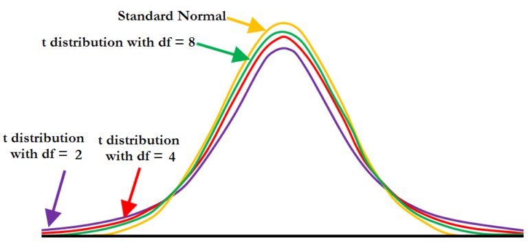
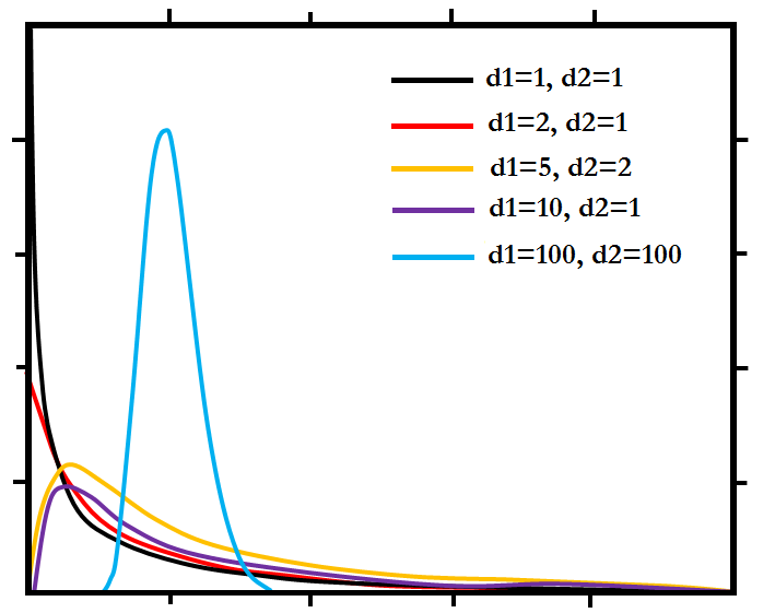
Parametric statistics are used to make inferences about population parameters i.e. so far we have been drawing random and representative samples from the population so that by performing statistical tests on these samples, some generalisation or inferences about the population can be drawn. Thus we use sample statistics to estimate population parameters and this is known as Parametric Statistics. So far we have used parametric statistics to find means, the difference between group means etc and have used various parametric tests such as t-Tests and F Tests etc. In all these cases we were able to draw inferences on the basis of Null Hypothesis significance testing. Also in all these tests, we assumed a certain sampling distribution such as T Distributions and F Distributions where each of these had a family of distributions where each of these family of distribution is selected based on the degrees of freedom which is based on the sample size.

Family of T distributions for different degrees of freedom — T Family of T Distributions (the distributions depend on the degrees of freedom, which is a function of the sample size).

Family of F distributions for ANOVA at different degrees of freedom — F Family of Distributions (for ANOVA) (the distribution depends upon the degrees of freedom, which is a function of the number of subjects in the group and the number of groups being compared).

Now all these inferences about the population are based on the sample distributions which have a lot of assumptions (such as homogeneity of variance assumption for ANOVA and Independent t-Test) and if the assumptions are not true and cannot be fixed (if assumptions are not true then some ‘tweaking’ or ‘fixes’ can be done such as using a restricted error term or changing the degrees of freedom so that parametric statistics can be used) then the parametric statistics are to be abandoned and a non-parametric approach is to be used.

Non-Parametric Statistics

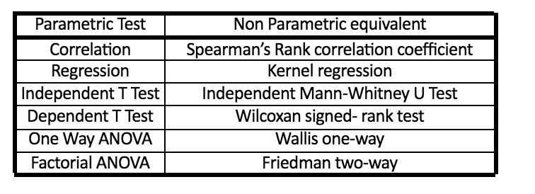
Non-Parametric Statistics don’t assume that the population of their sample have any particular characteristics (such as the population being normally distributed or having a linear relationship between predictors and the outcome). It is interesting to note that there are Non Parametric tests available for all the kind of parametric tests that have been discussed so far (Correlation, Z Test, t-Test, ANOVA) and one can use non-parametric procedures if required.

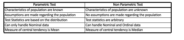
Table of non-parametric equivalents of parametric tests — Some Non-Parametric equivalents of Parametric Tests.

Table comparing parametric and non-parametric statistics — Some of the prominent differences between parametric and non-parametric statistics.

Thus when populations are skewed or the assumption required for the working of parametric statistics cannot be fulfilled then Non Parametric tests come very handy as they are very easy to understand and no assumptions are made regarding the population distribution. Also, Non-Parametric statistics uses median which is more effective when the data is skewed (Refer Measures of Central Tendency). Also, Non-Parametric Tests are effective when the sample size is not large enough. However one must note that some Non Parametric tests can only handle nominal or ordinal scaled data and are also not as efficient as parametric tests.

Understanding Chi-Square with an example

In this blog, one of the most useful non-parametric test is explored- the Chi-Square test.

Chi-square test uses two categorical variables (or nominally scaled variables) and is a non-parametric test because it makes no assumptions about the distribution of the sample while doing the Goodness of Fit test. Goodness of Fit test is used to check whether a given distribution fits the sample well or not (in other words if the sample data represents the data you would expect to find in the actual population or not) and is used in statistics such as the Chi-Square, Shapiro-Wilk, Kolmogorov-Smirnov etc.

An example will be very helpful to make you understand how the Chi-Square works.

We have two categorical variables- First one is the Country of Origin which has two levels- British and Americans. The second categorical variable is the Type of Sports which has three levels- Football (Soccer), Baseball and Cricket. We have a coaching centre where training for each of these sports is given. We have a sample dataset where the number of Britishers and Americans enrolling in different sports is known. We have to find if there is any relationship between the Country a person belongs and the Sports he chooses.

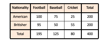
Observed frequencies table of Americans and Britishers enrolled in Football, Baseball and Cricket — The Observed Frequencies Table.

The way chi-square works is by comparing the data that we have collected (The Observed Frequencies Table) with the frequencies that it would have expected (Expected Frequencies table). This Expected Frequency table will have values that we would ‘expect’ in each cell by chance alone. These ‘expected values’ are simply calculated by taking the total count of that group (e.g. we want to calculate the expected value for Americans who would enrol for the sport- football. We take the total count of American (which here is 200) and divide it by the total number of samples (which in our example is 400) and multiplying this value by the total count of the other group in question which in our case will be 195 (the count of people enrolled in the sport- Football). Thus if we have to calculate the expected value for the number of American enrolled for Football, we will take the total number of Americans, the total number of people enrolled in Football and the total number of people in our sample and use these values to calculate the expected value. Thus the formula for this particular cell will be-

Expected value calculation for American Football cell

Similarly, we calculate expected values for every combination and end up with a table of Expected Frequencies.

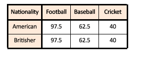
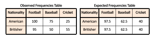
Expected frequencies table for Americans and Britishers across Football, Baseball and Cricket — Expected Frequencies table.

It will be interesting to see the comparison between our Observed Frequencies Table and Expected Frequencies Table.

It is interesting to notice how the values for Americans and Britishers for each sport has the same expected value, this happens because the sample size of the groups of the variable ‘Nationality’ is equal and with such an equal size, we expect that there will be equal number of Americans and Britishers for each sport. Here we can see that major change between the observed and expected values is for Baseball and Cricket while for Football, there isn’t much difference between the expected and the observed. The Observed Frequencies Table is the Contingency table. With chi-square, what we are performing here is the chi-square test of independence where we see if the number of cases (or the frequency) in each category (group or level) of each variable is dependent upon (contingent upon) the category (group or level) of the other variable or not. So what we basically test here is if the amount of people enrolling for Cricket is dependent upon their nationality i.e. of being a Brit or not.

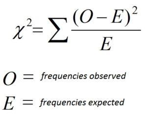
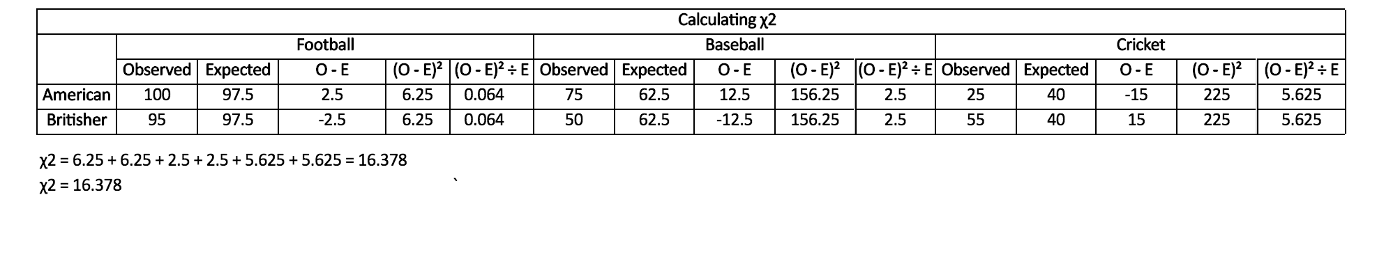
Now it's time for hypothesis testing through which we’ll be able to answer whether the difference in the frequencies is statistically significant or not and just like we came up with t-values for t-Test and F values for F Test, we have a chi-square test statistic (χ²). And the formula to calculate it is mentioned below-

Chi-square statistic formula, chi squared equals sum of observed minus expected squared over expected — Where O = frequencies observed and E = frequencies expected.

In this example, our value of chi-square statistic comes out to be 16.378.

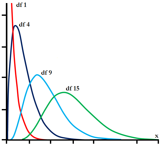
Now before looking into the chi-square table, we have to consider the degrees of freedom (just like we did before looking into t-Table or F Table) as the chi-square distribution is based upon the degrees of freedom (the way t and F distributions are based upon their degrees of freedom).

Family of chi-square distributions for different degrees of freedom — Chi-Square family of distributions.

Here the degrees of freedom is the number of groups. Here we have two categorical variable where one has two groups (Nationality: American and Britisher) and the other has three groups (Sports: Football, Baseball, Cricket). To put it simply, the degrees of freedom here is the Number of Rows of the contingency table minus 1 multiplied by the Number of Columns in the contingency table minus 1. In this example, the degree of freedom will be

df = (2−1) (3−1)
df = (1) (2)
df = 2

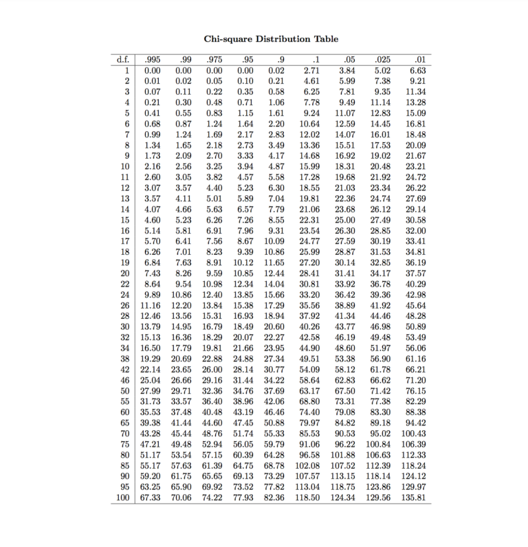
Now we can look at our chi-square table.

Chi-square critical value table for various degrees of freedom and significance levels

If we adopt an alpha level of 0.05, we get the critical χ² value of 5.99, and as our χ² value is larger than the critical value we conclude that our p-value is less than 0.05 and we can reject the Null Hypothesis and as always the Null Hypothesis states that there is no relationship between the two variables and the two variables are independent while the alternative hypothesis states otherwise. Thus we can say that the Nationality of a person did play a role in the choice of sports he enrolled in.

Chi-square distribution curve with the critical region shaded

Multiple chi-square distribution curves for different degrees of freedom — Chi-square distributions shift shape as the degrees of freedom change.

The chi-square is one of the most important and widely used non-parametric statistical tests. It is used when we want to compare two categorical variables. With the knowledge of basic statistics, we can proceed with preparing our data for modeling.