// important concepts

Z Scores, Z Test and Probability Distribution

In the previous blog concepts such as standard error and central Limit Theorem were explored giving us an idea how samples can take a similar shape of the population distribution and how sample’s mean can coincide with the mean of the population. On the basis of that understanding, in this blog post, few inferences will be drawn about the population by understanding how Z score, Z Test and probability distribution works.

Standardisation and Z scores

Standardisation means using the mean and the standard deviation to generate a standard score also known as the z-score to help us understand where an individual score falls in relation to the other score in the distribution. A z-score is a number that indicates how far above or below the mean a given score is in the distribution in the standard deviation units i.e. how many standard deviations a score is above or below the mean. If the raw score is above the mean then the z-score will be positive and if it falls below the mean then it will be negative. Standardisation thus is simply a process of converting raw scores in the distribution into standard deviation units or can say that it is a process of converting a raw observation into a z value. It allows us to calculate the probability of a score occurring within our normal distribution as well as enables us to compare two scores that are from different normal distributions. Here the Standard Normal Distribution has all the properties that a normal distribution has along with the mean being 0, standard deviation being 1 and the total area under the curve being one. Standardisation of data thus helps us by creating a standard normal distribution with the mean of the distribution being 0 and standard deviation being 1 making the data unit free and this helps us if we want to compare data that are on different scales (example- comparing Income and Time spent on phone calling).

The formula for calculating z score is-

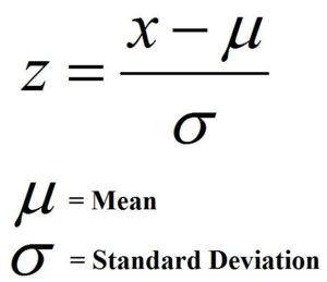
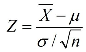
Here the x can be a raw score however if converting a sample mean into a z-score then the raw score is replaced by the sample mean and the standard deviation in the denominator is replaced by the standard error. The formula for the standard error here will be-

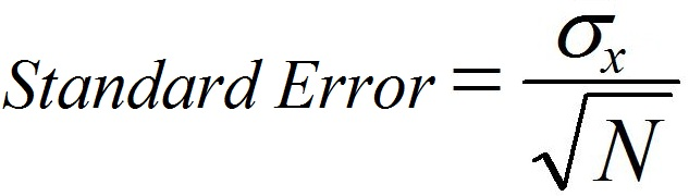
Thus the formula for calculating z score for a sample mean becomes

Examples

Below are a couple of questions and they have been answered by using z score. This will make it clear why and how z scores can be used.

Question 1- There is a class of 50 students and a Math exam is conducted. We assume that the data generated from the outcome of this exam is normally distributed (because of Central Limit Theorem). The exam which was of 100 marks had an outcome where the mean score was 60 out of 100 while the variation (fluctuation in the student’s marks) was of 15 (Standard Deviation).

Here the Question is if student-A scores 70 marks, did he score well? From how many students his marks are more and from how many students he scored fewer marks i.e. where his individual score falls in relation to the other score in the distribution. Secondly, what is the top 10% of the students?

And lastly, if student-A scored 72 marks in his Science exam, does it mean he scored less compared to his maths exam given the mean of the scores of Science exam is 68 and the standard deviation is 6.

Answer 1- To answer the first question, it may seem that marks of student-A are good because they are more than the average of the class but we have to keep the variation of marks in mind too so we see his marks in relation to where they lie in the distribution. We can use probability distributions. Probability distribution helps us in providing a score for a value for a given distribution. In this example, we have presumed that the marks of the students are normally distributed therefore we use standard normal distribution and find its related z-score.

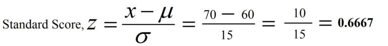
Now, to find where the score of student A falls in comparison to the other students in the class, we calculate the marks of student-A in terms of z score. Here the mean is 60, the standard deviation is 15 and the individual’s score is 70. So the z score of student A will be 0.6667.

Now we use the Standard Normal Distribution table to find the probability of a score being greater or less than our z score of 0.666. The y-axis in the table highlights the first two digits of our z-score and the x-axis the second decimal place.

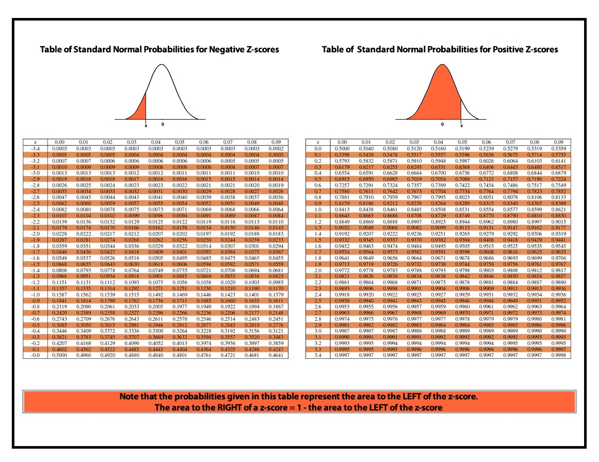
Here we use the above table (Right) and find the value of the z score is 0.7486 and if we multiply it by 100 then it comes out to be 74.86. This means that around 75% of the data is on the left of our score i.e. almost 75% scored fewer marks than student A. Now to find how many students scored more than student A, we can either use the Inverse Standard Normal Distribution table (or consider the z-value to be negative and use Table of Standard Normal Probabilities for Negative Z-scores) which will tell out about the area under the curve on the right side of our z score of 0.667 when plotted on a standard normal distribution, or we can simply subtract 100 out of 74.86 and say that 25.15% or almost around 25% of the students scored higher marks than student A.

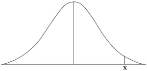
For answering the second question, which requires us to know the top 10% of the students, we can presume a point X on our standard normal distribution, and find the value of X in terms of z score on whose right side 10% of the data lies or is under the distribution curve.

We can look at the Standard Normal Distribution table and try to find score closest to 0.9000 and we end up finding the closest value of 0.8997 and by looking at the x and y-axis we compute that the z score will be of 1.28 (1.2 (y-axis) + 0.08 (x-axis)).

Now we have the z score, mean and standard deviation and we can easily find the score.

z = x − μ / σ (formula to find z score where x is known)

x = μ + (z) (σ) (formula to find x when z score is known)

x = 60 + (1.28) (15)

x = 60 + (1.28 × 15)

x = 60 + 19.2

x = 79.2

Thus the students who score more than 79.2 are those students that are in the top 10% of the class.

To find out the answer for the last question, where we need to find if Student-A scored more on his Science exam, we have to compute the z score of his Science marks too and compare it with the marks of his Maths Exam to find if he has actually fared better or not.

To find the z score of his Science marks we subtract the mean marks of his science class with his individual marks and divide it with the deviation (standard deviation) found in his science exam scores (72-68/6) which comes out to be 0.67 which is the same as what was found in his Math exam. Thus student-A actually didn’t score any better in his science exam.

There are various other questions which can help us understand how useful z scores can be to us.

Question 2- What is the percentage of students who scored marks between 567 and 617 when the mean of such normal distribution is 517 and the standard deviation is 100.

Answer 2- Here we first find the z score of both the marks.

z = x − μ / σ

Marks 1: 567-517/100 = 0.50

Marks 2: 617-517/100 = 1.00

Now we look at the Standard Normal Distribution table to find the area under the curve for each score. So the percentage of students who score less than 567 (i.e. the percentage of data to the left of z score 0.50 when plotted on a standard normal distribution) is 0.6916 i.e. 69.15%. Similarly, for a score of 617, it is 84.13%. Therefore the percentage of students who scored between 567 and 617 is (0.8413-0.6915) 14.98%.

Question 3- What is the percentage of students who scored more than 130 in a Math test where the mean of the normal distribution was 100 and the standard deviation was 15.

Answer- There are two ways of doing this- By calculating the area under the curve using Standard Normal Distribution table or by using Inverse Standard Normal Distribution.

If we use Standard Normal Distribution table, we can find the percentage students who scored less than 130 (data to the left of the z score) and then subtract it by 100 to find the students who scored more than 130.

Here we will use the value of z score as it is (130-100/15 = 2.00). Now if we look at the Standard Normal Distribution, the students who scored less than 130 comes out to be 97.72%. Therefore 2.28% (97.72-100) of the student scored more than 130.

Another way is by using the Table of Standard Normal Probabilities for Negative Z-scores. Here we consider the z score value to be of negative i.e. -2.00 to find the data to the right of the z score if plotted on a standard normal distribution, and when we look at the Table of Standard Normal Probabilities for Negative Z-scores to find the percentage of students who scored more than 130 directly which comes out to be 2.28%.

Probability Distribution and Z Score

We can now understand how we can find probabilities using the Standard Normal Distribution. Here the term probability means area and as discussed above, the total area of a standard normal distribution is 1. So here the probabilities that we compute will always be less than 1.

Examples

Below are a couple of questions that will help in understanding how z scores and probability distribution works to find probabilities.

Question 1- What is the probability that z is less than -1.32 on a Standard Normal Distribution.

Answer- Here to find the P(z < -1.32) we have to first consider the Table of Standard Normal Probabilities for Negative Z-scores as our score is negative (i.e. to the left of the mean). Also as we have to find the probability of z being less than -1.32, we will find out the area to the left of the z score. When we use the table of Standard Normal Probabilities for Negative Z-scores, we find that the area under the curve comes out to be 9.34% (value found in the table being 0.0934).

Question 2- What is the probability that z is more than -1.32 on a Standard Normal Distribution.

Answer- We have to find P(z > -1.32) and here also we use the Table of Standard Normal Probabilities for Negative Z-scores, but this time as we have to find the probability of z being more than -1.32, therefore we have to find the area to the right of our z score, and as our table only provide us with the area to the left, we can simply subtract the value by 1 (Total area under the curve) to find out the area to the right which will be (1-0.0934 = 0.9066) 90.66%. Thus the probability of having a z score more than -1.32 is 90.66%.

Question 3- What is the probability of z being in between -1.28 and 0.72 on a standard normal distribution.

Answer- The solution to this is very simple. We find the area to the left of -1.28 and 0.72 and then subtract them to find the area in between. So the area to the left of -1.28 (using Table of Standard Normal Probabilities for Negative Z-scores) is 0.1003 i.e. 10.03% while the area to the left of 0.72 (using Table of Standard Normal Probabilities for Positive Z-scores) is 0.7643 i.e. 76.43%. Therefore the area between them will be i.e. 66.39%.

Question 4- A similar more practical question is, What is the probability of a randomly selected adult American female is taller than 170.5 cm when the mean is 162.2 cm and the standard deviation is of 6.8 cm.

Answer - Here we have to find the z score of 170.5 cm and then have to find the area to the right of this z score. So here the z score will be 1.22. The area to the left will be 88.88%, therefore the area to the right will be 1-88.88 i.e. 11.12%. So the probability of finding such a female is 11.12%. (Here we can also infer that this z score of 1.22 means that 170.5 is 1.22 standard deviation above the mean of 162.2 as z score simply tells us how many standard deviations a value is above or below its mean.)

Z Test

Z Test is a hypothesis test which is based on Z-statistic, which follows the standard normal distribution under the null hypothesis. The above discussed Z-value is a “test statistic for Z-tests that measures the difference between an observed statistic and its hypothesized population parameter in units of the standard deviation.”

Z Tests are used in various scenarios such as one sample z-test, testing the mean of a normally distributed population where the standard deviation is known. It is also used during Regression to find if the predictor (independent) variables have a significant impact on our dependent variable or not. Z Test is also used to do a normal approximation for tests of Poisson rate and tests of proportions. Thus Z-Test is used for Hypothesis testing in scenarios-

• Testing means where population is normal, sample size is large and variance is known
• Testing Difference of means where population is normal, sample size is large and variance is known
• Testing of Proportions or difference between proportions (used for categorical / qualitative data)

Z Test is used in hypothesis testing and in the next blog, z values in Z test will be used to perform hypothesis testing where probabilities will be calculated to accept or reject a hypothesis.

The above-mentioned question (Question 4 under ‘Probability Distribution and Z Score’) used the z values for finding probabilities. More about Hypothesis Testing is there in the next blog, but to give you some idea, the same question mentioned above under hypothesis testing will look something like this-

The average height of an American female is 162.2 cm with a standard deviation of 6.8 cm. A recent survey conducted on American women having a sample size of 200 women found that the average height is of 170.5 cm. Has the height of average American women increased?

Here we will use the same calculation and will use a Z-test but the way we draw inference will be different and will use terms such as Null Hypothesis, Alternative Hypothesis, P-value etc (More about this under Hypothesis Testing).

Other Probability Distributions

Apart from the most commonly used probability distribution- The Normal Distribution (aka Gaussian Distribution), there are many other kinds of Probability Distributions.

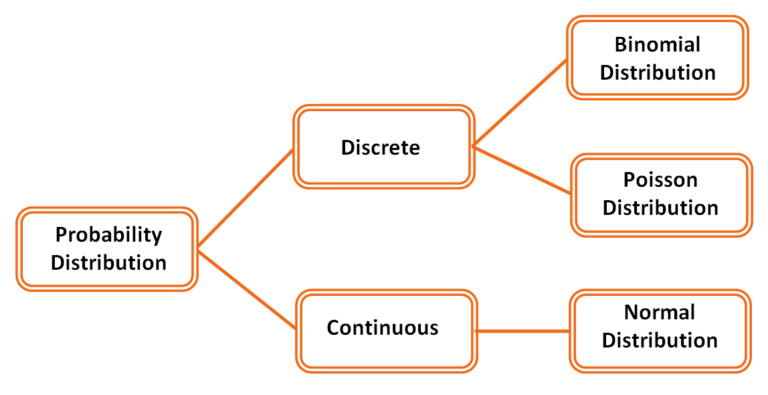
Other kinds of probability distributions can be for example-

Binomial: Here there are only two potential outcomes with the probability of success being same across all trials with each trial being independent. Example- Distribution generated from tossing a coin.

Poisson: It is a discrete distribution. It describes the number of events occurring in a fixed time interval or region of opportunity. Example- How many tourists visit a monument site which is open from 9 AM to 5 PM.

Other distributions can be Hypergeometric which is somewhat like Binomial, however, the probability is not exactly 50-50% percent for an outcome but fluctuates throughout. An example can be - Out of 5 cards how many spades can be there where with each pick, the probability fluctuates. There are many such distributions that you should further explore such as Log Normal, Chi-squared, Gamma, Beta, Weibull, Exponential, Negative Binomial etc.

In this blog post, certain inferences were drawn and mere features of the data weren’t described. In the next blog, the concepts explained in this post will be put to use.