// feature construction

Binning

Binning is simply the process of creating new categorical variables from numerical variables. Binning can also be termed as discretization, which is “the process of transferring continuous functions, models, variables, and equations into discrete counterparts.”

Use of Binning

Examples of binning can be found everywhere, such as where the age of people of a city is given as 0-9, 10-20, 21-39, 40-59, 60-89, 90+. The process of binning lies somewhere between feature creation and feature transformation, as we can also say that binning is where we transform our numerical feature into a categorical feature. This transformation can be required due to various reasons. Sometimes the analyst has to read between the lines and consider certain effects or patterns in data caused by the involvement of humans, and then formulate implementation strategies. For example, if we are analyzing the marks of students of grade 10 and find that there is a correlation between their IQ level and marks, new study material or methods cannot be created for each different student with a different IQ. Here we can bin the IQ of students into 4 groups and come up with a new specialized method of study for each of the groups. Thus the implementation part also has to be considered, which helps us understand when each step of Feature Engineering is to be performed.

Processes like binning also help in improving the reliability of various models, especially linear and predictive models, as they help in reducing noise (unexplained/random data points) and non-linearity found in the data. Interestingly, just like other transformation techniques, binning also helps to control the effect of outliers to an extent, as especially during supervised binning (mentioned below), where a decision tree algorithm is used, the effects of outliers are controlled to an extent. Binning can also help in the detection of outliers. Binning helps in the reduction of overfitting, which is a common problem that occurs during modeling, as through binning the model doesn’t try to draw different inferences from values that are very close to each other.

Note how some of these characteristics (helping with non-linear relationships, outliers, etc.) found in Feature Transformation techniques can also be found in binning, and thus we can say that binning is also a form of variable transformation, although in this section it has been included under Feature Construction, as a new variable is also being formed here.

Types of Binning

Binning can be categorized into two types: Unsupervised and Supervised.

Supervised Binning

In supervised binning, the target variable (commonly referred to as the ‘Y variable’) is also considered, and binning is done keeping the various categories of the Y variable (also known as the class label, which is the discrete attribute whose value we want to predict) in mind. One of the most common techniques is Entropy-based binning. Entropy is a method used by ID3, which is the core algorithm for building Decision Trees, by splitting the variables where maximum information is gained, with these splits being based on the class label, making these bins correspond to the same class label. (More on Entropy is discussed in the blog on Decision Trees.)

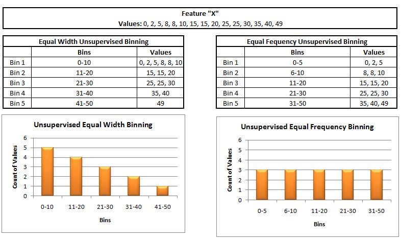
Unsupervised Binning

This is the simplest and easiest form of binning, where the target variable is not considered, and only the values of a variable are considered to divide and convert them into different categories. The most commonly used among Unsupervised Binning methods is Equal Width Binning, where the values of a feature are divided into ‘k intervals of equal size,’ with the interval size being uniform throughout. Another type of Unsupervised Binning is where, for example, we have a variable which has 10 values, and binning is done by dividing these values into k groups, with each group having roughly the same count of values, so if the feature has 10 values and we form 5 segments, then each segment or group will have 2 values. Such a way of Unsupervised Binning is known as Equal Frequency Binning. Bar graphs of such a binning process can be made by the use of frequency tables.

Ranking and Quantiles

Other methods such as Ranks and Quantiles can also be used for binning. Ranking can be done by sorting the data and giving ranks to each value, based on the position of these values, with these ranks indicating the value’s size or weight in relation to the other values of the same feature. Quantiles can be used for binning by the use of Quartiles, Quintiles, Percentiles, etc. (more on this under Descriptive Analysis). Both these methods have their limitations, with Ranking having the drawback that it will give separate ranks to the same values (due to duplication), and can cause the same values to have a different rank if there is any alteration in the data, which is also a drawback of the Quantile method.

Thus, binning makes sense when the data can be divided into neat ranges, where all values under a bucket/bin have a common characteristic. However, binning your features is not a good idea if the buckets don’t make sense or high precision is required.