// feature construction

Encoding

In the previous blog, Binning was explored, which is the creation of new variables by transforming numerical variables into categorical variables. The opposite of Binning can be termed Encoding, where new variables are created by transforming categorical variables into numerical variables. This is done mainly because most machine learning algorithms cannot read categorical data and require it to be numerical in nature. The simplest example can be of gender, where to a modeling method such as Linear Regression or SVM, the terms ‘Male’ and ‘Female’ won’t make any sense, and to make such a variable useful to a learning algorithm, each of these terms (categories) is transformed into a binary attribute (0 and 1), so here we can have 0 representing males and 1 representing females, and by doing so, the algorithm can take the values into consideration.

Methods of Encoding

There are mainly two methods of encoding: Binary Encoding and Target Based Encoding.

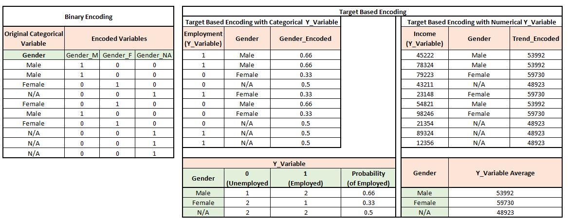
Binary Encoding

In Binary Encoding, we use binary values to indicate whether a category is present or not. Here, for each category of a feature, a separate variable is created having values 0 and 1, where the presence of a category is denoted by 1 while absence is generally denoted by 0. This causes a potential problem of increase in the dimensions of data, especially if a variable has a very large number of categories, causing that many new variables to be formed. Here the curse of dimensionality takes place, which basically means that when the data is in very high dimensions, the model is not able to perform and predict accurately. However, if the dimensions are too low, then it can cause underfitting, and the model may require additional information (i.e. some extra variables); however, again, if we add a lot of variables without adding any information (not able to explain the variance of our target variable with our new additional variable), it will lead to adverse effects and will decrease the model’s accuracy. Thus this tremendous increase in the dimension of data due to encoding can cause various problems during the modeling process.

Target Based Encoding

The other method is Target Based Encoding, where, unlike Binary Encoding, separate variables for each category of a feature are not created; rather, a single separate numerical feature is created for a categorical variable, where for each category, its corresponding probability of the target label is provided. For example, if we have a dataset where we have two variables, Gender and Employment, with Gender being the independent variable having two categories ‘Male’ and ‘Female,’ and the ‘Y Variable’ or dependent variable being Employment, having two target labels, 0 for Unemployed and 1 for Employed: here, in the new numerical variable for the feature Gender, in place of the category ‘Male,’ its corresponding probability of the target will be provided. A similar process will be done for the other category. However, if the Y variable is numerical, then the average of the target variable is taken. Target Based Encoding is not as powerful when compared to Binary Encoding, is dependent on the distribution of the target labels, and is less commonly used than Binary Encoding.

Scalar Encoder vs. One Hot Encoding vs. Dummy Variables

Encoding through Scalar Encoder

A Scalar Encoder is used when there are only two categories in a feature. For example, if we have a dataset with a feature such as Gender, where there are only two categories, ‘Male’ and ‘Female,’ a Scalar Encoder can be used by giving Males a representative value of 0 and Females a value of 1, or vice versa. Here the dimensions of the dataset are not increased drastically, and can be maintained by dropping the categorical variable once it has been encoded.

One Hot Encoding

This term is commonly used in machine learning models. Here, for each category of a feature, a separate variable is created having values 0 and 1, which works like an ‘on and off switch,’ where 1 is assigned if a particular category is present and 0 if it is not. So if there is a feature having 10 (N) categories, 10 (N) variables are created by One Hot Encoding.

Encoding through Dummy Variables

The only difference between One Hot Encoding and Dummy Variables is that, unlike One Hot Encoding, N-1 variables are created. Here one of the dummy variables is left out, as it serves as the base assumption, to avoid perfect multicollinearity among the dataset. It can be said that the term Dummy Variable comes from statistics, while One Hot Encoding is from computer science, which in turn is borrowed from electronics.

As mentioned above, the major problem with these types of encoding methods (One Hot and Dummy Variable) is that they can lead to very high dimensions, which can cause overfitting or can make the model computationally expensive. The high cardinality and the curse of dimensionality caused by encoding can be addressed by using dimensionality reduction techniques such as PCA.

Other Methods

Label Encoder

Label Encoding is a very simple method of encoding where we encode labels with values between 0 and n_classes-1. For example, if we have a feature ‘colours’ having 3 categories, Blue, Green, and Red, Label Encoder provides numeric values for each of the categories, so, for example, Blue is given 0, Green is given 1, and Red is given 2. However, this method of encoding poses significant problems, such as when the values don’t have any natural ordering (if colors don’t have any weight); these encoded values can then provide misleading results, as any mean derived from such an encoded variable will be wrong, and if such values are used by learning algorithms, then incorrect predictions will be made by the model.

Simple Replace

Sometimes certain numerals are provided in the form of text. For example, we have a dataset where the number of cars owned by a household is provided as ‘one,’ ‘two,’ ‘three’ rather than 1, 2, 3. In such situations, the variable can simply be transformed into a numerical variable by finding such text and replacing it with its numerical equivalent.

Feature Construction can be done by encoding through the various methods discussed above, each with its own advantages and disadvantages. Among all the encoding methods discussed, One Hot Encoding is the most popular and commonly used, however, the curse of dimensionality must be kept in mind when using it.