// anomaly detection

Unsupervised Anomaly Detection

Outliers can create problems in the working of various modeling algorithms and need to be addressed especially for modeling algorithms such as K Nearest Neighbour, which is a distance-based algorithm. Various ways of handling outliers have been discussed under Outlier Treatment. However, there is a machine learning method known as Anomaly Detection that can be used to detect the outliers. Here the definition of outliers can be understood as observations that are inconsistent with the majority of the remaining data. Therefore, here various machine learning algorithms try to find the observations that deviate from the other observations, which can lead us to think that they might be an outlier. There are mainly three types of Anomaly Detection setups - Supervised, Semi-supervised and Unsupervised - and in this blog, Unsupervised Anomaly Detection will be discussed.

Introduction to Anomalies

The most common scenario is where one has to work with a dataset with less domain knowledge about it, and in such a situation, identifying the outliers and determining if the dataset contains outliers or not becomes extremely difficult. As discussed in the introduction of this section, finding anomalies under such a setup is very tough, as the data at hand can be good or it can in all possibility be bad and riddled with outliers, noise and anomalies. Here we can only presume that our data has a limited number of outliers.

The unsupervised anomaly detection method works on the principle that the data points that are rare can be suspected of being an anomaly. To understand this properly let us take an example. Suppose we have a dataset which has two features with 2000 samples, and when the data is plotted on the x and y-axis, we come up with the following graph:

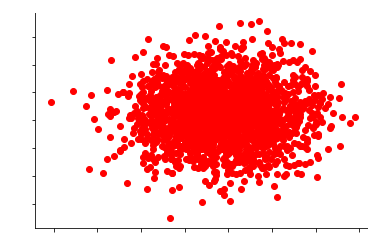
Now if we look at the graph, we can see that all 2000 data points make a cluster. We can now understand how the idea of a data point being rare will function to find the anomalies. If we try to estimate the density of this dataset and once estimated, we score each of these 2000 data points by the probability of observing them under the dense region. Thus, out of these data points, those data points can be labelled as anomalies who have a very low probability, meaning that they are (figuratively speaking) away from the dense region/cluster. This probability is nothing but a quantified value of anomaly.

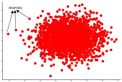
By only looking at the image, we can see that certain data points fit into the category of being an anomaly, as they seem rare and are inconsistent with the majority of the remaining data.

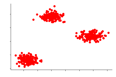
However, many times the data forms more than one cluster, and under such cases, our data may look something like this:

There are various kinds of Unsupervised Anomaly Detection methods, such as Kernel Density Estimation, One-Class Support Vector Machines, Isolation Forests, Self Organising Maps, C Means (Fuzzy C Means), Local Outlier Factor, K-Means, Unsupervised Niche Clustering (UNC) etc. In this blog, three methods - Kernel Density Estimation, One-Class Support Vector Machines and Isolation Forests - have been discussed, and rather than getting into their mathematical details, we will see how these methods work on the data mentioned above.

Kernel Density Estimation

Kernel Density is a non-parametric way of estimating densities. We can easily understand it by applying this method to our data. Suppose our data, when plotted on the x and y-axis, shows 3 clusters. We first estimate the densities of these clusters by fitting a model using a kernel. We now look for log probabilities, which are single values given to each data point. These log probabilities indicate the log-likelihood of a data point being observed under the density estimated during the fit procedure. We can then remove those data points that don't fall under the estimated density. Here the smaller the value of the log-likelihood is, the rarer the sample is. Thus we end up finding the anomalies.

There are multiple ways of estimating the densities of the data points. We can use histograms, which is a completely non-parametric way where we come up with bins. All the data points then fall into these bins, and the bins that have a very low number of data points are marked as an anomaly. However, they suffer from a major issue of the increase in the number of bins, as when the data is in high dimension, these bins can increase exponentially. The other commonly used method is Gaussian Mixture Models. It is a common model used for Generative Unsupervised Learning, i.e. Clustering, particularly Expectation Maximization Clustering. A Gaussian distribution has been explained under the section Basic Statistics. Here, Gaussian Mixture Models are probabilistic models that represent multimodal normally distributed distributions, where we describe our data as a mixture of Gaussians. This method of estimating density is commonly used in Anomaly Detection, as it is better adaptive to the data. All these Density Estimation methods provide us with values that indicate how unlikely it is for a data point to fall under the density region, and these values are turned into anomaly scores.

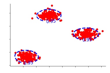
Let's first take a look at what we get after applying Kernel Density Estimation on our data.

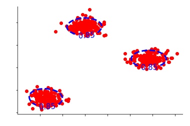
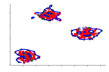
We use the density function according to which all the data points that are inside these blue circles are under the high-density region and are normal observations, while all the data points outside this circle are anomalies. Here we have set the quantile at 85%, which means that we have constructed the data in such a way that 15% of the data remains outside the circle. This leads us to the most important parameter that we need to define to perform Kernel Density Estimation, which is the assumption that 15% of our data is contaminated. Thus, we require setting a threshold about what fraction of data is to be considered as an anomaly.

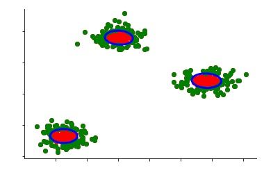
If we change this threshold to say 95%, then only 5% of the data will be considered as an anomaly.

Thus, this method is very sensitive to the threshold value. Also, an implicit parameter here is the Euclidean distance, as just like K-Means, we need some ground metric to compare the distances of different samples, and as we have discussed multiple times so far, the methods that require a distance metric to function come with their own set of problems which need to be addressed.

Also, this method doesn't work well when the data is in high dimension, as with all distance-based models, when the data is in very high dimensions, the data space is almost empty even if we have a lot of data points, which makes the task of estimating density very difficult.

One Class Support Vector Machines

Support Vector Machines has been discussed in its separate blog. Here we discuss One-Class Support Vector Machines, which are extensions of the earlier discussed Binary SVM, where one class basically means that we are working in an unsupervised setup. Here we find a decision function which can be non-linear and based on kernels. The decision function here is sparse in the number of samples, which basically means that we have very few samples that allow us to separate what is outside the normal region from what is inside. The One Class SVM follows the same idea of density regions, where points falling inside a certain region are termed as normal while the data points outside are termed as an anomaly; however, they are better than Kernel Density, as Kernel Density doesn't work well in very high dimensions, whereas One Class SVM estimates a decision function which works well even in high dimensions. Therefore, unlike Kernel Density, which estimates density, One Class SVM comes up with a decision function that simply tells you whether the value of a data point is low enough to be considered an anomaly or not.

Here, too, the most basic and important parameter we use is the threshold value, i.e. the fraction of data that we presume to be contaminated. If we set our threshold to 50%, then half of our data will be considered as an anomaly.

However, if we take a more decent number, say 5%, then 5% of our data will be considered as an anomaly.

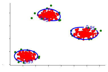
Another important parameter here is gamma, which is a commonly used parameter in kernel-based SVMs. Here, gamma can be understood as a bandwidth parameter of the kernel. Therefore, if we use a very small value of gamma, we will end up having a very wide Gaussian kernel, which means that we will end up modeling our data with a single big mode. However, in many cases, the data is not a simple Gaussian distribution but a mixture of Gaussians, and in our case, we can see that it forms multiple clusters of data which each have a Gaussian blob. Therefore, we don't have a single mode but have a multi-modal distribution, so a single big mode is not required.

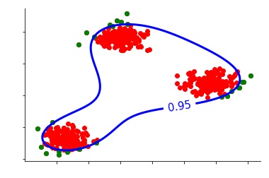
Thus we need to increase gamma in order to achieve an optimum bandwidth of the kernel that can accommodate the three clusters of data.

However, if we increase the value of gamma a bit too much, then we will come up with a very complex decision function, as the bandwidth of the kernel will be so low that it considers too many clusters of data that may not even be there.

Thus, here we don't only have to worry about the percentage of data to be considered as an anomaly, but also the gamma parameter, which greatly affects the result.

Isolation Forest

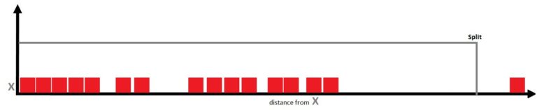
This method of Anomaly Detection is based on trees. As discussed in Decision Trees, we know that it is a very powerful method where space is divided using various partitioning methods. This partitioning of data is done by making splits along the axis direction. We use this technique to isolate certain data points - for example, if we have only one feature, then all these data points can lie on the x-axis. We can then determine the data point which is far from all the other data points and split the axis in a way that the data point away from the other data points is on the other side of the divide.

Here the strategy is to find the anomaly in very few decisions, i.e. few splits. In this method, we construct a number of random trees, then take a random feature and a random threshold, and if the data point is in a far, rare location of the data space, then by this random splitting it will be isolated.

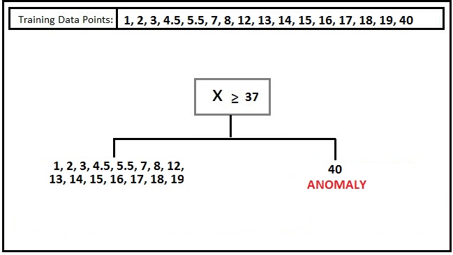
Thus, here we build random trees and see, on average, how many splits it requires to isolate the sample. If we find the optimum depth, then the isolated sample should be alone in a leaf after a few splits. We build multiple trees as we try to find the average number of splits required to isolate a sample, as doing this provides stability to the process. The Isolation Forest uses this method and comes up with values for different data points that indicate the ‘level of anomaly or abnormality’.

Here, apart from the amount of data that we want to classify as an anomaly, the other single most important parameter is the number of decision trees. If we use too small a number, then we make the decision boundary too complex; therefore, we add a number of trees to regularise the decision function. Thus, by adding more trees, we have more data to average out from, which provides more stability to the model. However, all of this follows the bias-variance principle. Here, a low value for the number of trees makes the decision function more complex and less generalized, while a higher number of trees smooths and stabilises it; beyond a certain point, adding more trees yields diminishing returns rather than a better fit.

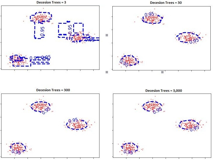
However, in this scenario, with a high number of decision trees, the concern is not of underfitting but of the running time and computation cost, as after a certain number of decision trees, any addition of them will not benefit the solution by much. It might not lead to underfitting but will lead to wastage of resources (time and other computational costs).

There are various methods of outlier detection and treatment discussed in the blog Outlier Treatment, where different statistical tools can be used to identify and treat the outliers. However, in this blog, more sophisticated methods of finding the outliers were explored. Here various unsupervised models can be put to use to identify the outliers, and then these outliers can be treated through the methods mentioned in Outlier Treatment.