// application · python

Classification Problems in Python

In the Theory Section of Modeling, various classification algorithms are explored. In this blog post, all those algorithms will be put to use using Python.

Importing Libraries and Preparing Dataset

We will be using the famous Titanic Dataset available on Kaggle for running the various Supervised-Classification modeling algorithms (only the train_data dataset is being used). The dependent variable here is a binary variable - Survived. Our objective is to predict the survival rate of the passengers travelling on the Titanic. Note that before using the dataset for creating classification models we need to perform some steps of pre-processing.

Importing Libraries

We begin by importing the libraries for operations on arrays and data frames.

import numpy as np
import pandas as pd
import matplotlib.pyplot as plt
%matplotlib inline

We import the library for splitting the dataset.

from sklearn.model_selection import train_test_split

We import the library for computing the accuracy score of the models.

from sklearn import metrics

We also import the libraries for tuning of parameters.

from sklearn.model_selection import GridSearchCV
from sklearn.model_selection import RandomizedSearchCV
from scipy.stats import uniform
from scipy.stats import randint as sp_randint

Importing Dataset

The Titanic dataset will be used for creating all the classification models.

Titanic1 = pd.read_csv('C:/Users/user/Desktop/Data Sets/Feature Reduction Datasets/Titanic1.csv')
Titanic1.head()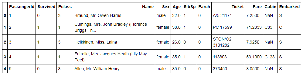

Show full table ▾

Missing Value Treatment

We check for missing values in the dataset.

Titanic1.isnull().sum()

We find that we have missing values in the variables Age, Embarked and Cabin, however we are mainly concerned with Age and Embarked.

We check the distribution of the Age variable.

Titanic1.hist(column="Age",figsize=(8,5),bins=15,density=True,stacked=True, color='orange')
Titanic1['Age'].plot(kind='density',color='blue')
plt.xlim(-10,85)

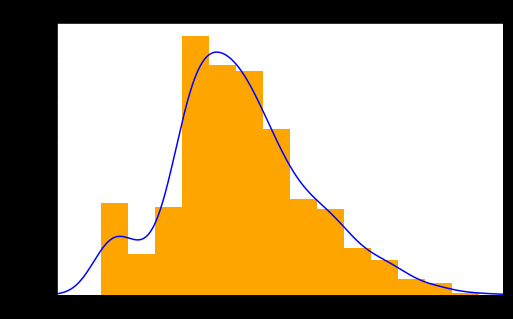
As the distribution of the variable is not quite normal and seems a bit skewed, we take the median to impute the missing values rather than considering the mean.

We first calculate the mean of the variable so that we can compare its value with the median.

Mean_Age = Titanic1['Age'].mean(skipna=True)
Mean_Age

We now calculate the Median Age.

Median_Age = Titanic1['Age'].median(skipna=True)
Median_Age

We find that the mean is approximately 30 while the Median is 28.

We also have missing values in the Embarked variable, and as it is a categorical variable we consider the mode. However, we first check the number of levels present in this variable along with their count.

Titanic1['Embarked'].value_counts()

We perform Mean and Mode Imputation along with dropping the Cabin variable as it will not be of much use for our analysis.

TitanicD = Titanic1.copy()
TitanicD["Age"].fillna(Titanic1["Age"].median(skipna=True), inplace=True)
TitanicD["Embarked"].fillna(Titanic1['Embarked'].value_counts().idxmax(), inplace=True)

We drop the Cabin variable and see how the data looks as of now.

TitanicD.drop('Cabin', axis=1, inplace=True)
TitanicD.head()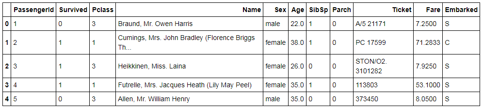

Show full table ▾

We drop the other variables which may not be of much use to our analysis.

TitanicD1 = TitanicD.drop(['PassengerId','Name','Ticket'],axis=1)

Dummy Variable Creation

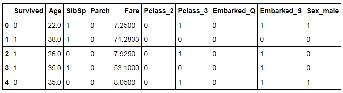
We create dummy variables for the categorical variables Pclass, Sex and Embarked.

TitanicD1 =pd.get_dummies(TitanicD1, columns=["Pclass","Embarked","Sex"],drop_first=True)
TitanicD1.head()

Show full table ▾

Train and Test Split

We will now split our dataset into train and test using the train_test_split function.

TitanicD1.to_excel('C:/Users/Datavedas/Desktop/Data Sets/Logistic Regression/TitanicD1.xls')
train_set,test_set = train_test_split(TitanicD1,test_size=0.3,random_state=123)
X_T = TitanicD1[['Age', 'SibSp', 'Parch', 'Fare', 'Pclass_2', 'Pclass_3','Embarked_Q', 'Embarked_S', 'Sex_male']]
Y_T = TitanicD1['Survived']
X_train,X_test,Y_train,Y_test=train_test_split(X_T,Y_T,test_size=0.3,random_state=123)

The Train Dataset.

train_set.head()

Show full table ▾

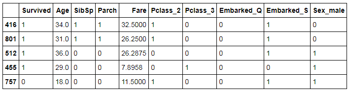
We export the Train Dataset.

train_set.to_excel('C:/Users/user/Desktop/Data Sets/Logistic Regression/train_set.xls')

The Test Dataset.

test_set.head()

Show full table ▾

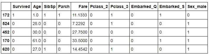
We export the Test Dataset.

test_set.to_excel('C:/Users/Natasha/Desktop/Data Sets/Logistic Regression/test_set.xls')

The Process of Creating Classification Models

In a typical case, we follow the following steps for creating a classification model:

• Step 1: Import packages required to run the particular model.
• Step 2: Fit the model on the Train dataset.
• Step 3: Predict the values on the Test dataset.
• Step 4: Compute the Accuracy score for the model.

We also perform tuning of the hyperparameters, which is done to improve the accuracy of our model and save it from overfitting. There are mainly three ways to tune these parameters: Grid Search, Random Search and Bayesian Optimization. In this blog, we will be tuning our parameters using the first two methods and see how the accuracy score gets affected by it. We will be using Grid Search/Random Search that fits the best model (i.e., model with best parameter values) on the train dataset and predict the value on the test dataset. It is important to understand the difference between Grid Search and Random Search.

In Random Search, when dealing with continuous parameters, it is important to specify a continuous distribution of plausible parameters to take full advantage of the randomization. This way, increasing n_iter will always lead to a finer search. For each parameter, we give a range of plausible values of hyperparameters. Unlike GridSearchCV, not all parameter values are tried out, but rather a fixed number of parameter settings is sampled from the specified distributions. The number of parameter settings that are to be tried is declared through n_iter.

The GridSearchCV means Grid Search Cross-Validation, wherein you can tell the program to run grid search with cross-validation. In grid search cross-validation, all combinations of parameters are searched to find the best model. The cross-validation command in the code follows a k-fold cross-validation process. Here our dataset is divided into train, validation and test set. After finding the best parameter values using Grid Search for the model, we predict the survival rate on the test dataset, i.e. a kind of unseen dataset. Cross-validation helps in avoiding the problem of overfitting of the model. Please refer to Model Validation Techniques under the Theory Section for a better understanding of the concept. The concept of Hyper-Parameter tuning with cross-validation is discussed in Model Validation in Python under the Application Section.

In this blog, we will perform Grid Search and Random Search without explicitly mentioning the number of folds required for cross-validation. However, it is important to note that by default, Grid Search and Random Search perform a minimum of three-fold cross-validation when tuning parameters.

Classification Algorithms

In the Theory Section of Classification Problems, we have explored a lot of classification algorithms and in this blog, we will create models using those algorithms to predict the survivability of a person present on the Titanic. We will be creating classification models using the following methods/algorithms:

• Logistic Regression
• Regularized Logistic Regression
• Decision Tree Classifier
• KNN
• SVM
• ANN
• Naive Bayes
• Bagging Classifier (Ensemble)
• Random Forest Classifier (Ensemble)
• AdaBoosting Classifier (Ensemble)
• Gradient Boosting Classifier (Ensemble)
• Xgboost Classifier (Ensemble)
• Stacking (Ensemble)

Logistic Regression

To understand how Logistic Regression works, refer to the blog on Logistic Regression in the Theory Section. In this blog post, we will use Logistic Regression algorithm to predict if a person will survive or not.

Import Libraries

We begin by importing statsmodel for running a simple logistic regression.

import statsmodels.formula.api as smf

Splitting the Dataset

The next step is to split the dataset into train and test. The ratio can be 60:40 or 75:25 as per your requirement. Here we will be taking the ratio of 70:30, where 30% is the test dataset. In Python, test_size indicates the percentage for the test dataset.

from sklearn.model_selection import train_test_split
train_set,test_set = train_test_split(TitanicD1,test_size=0.3,random_state=123)

Note: random_state is like the seed in R, the initial value to begin the process of random selection.

Running the Simple Logistic Model on Train Dataset

We will now run the model for logistic regression on the train dataset and predict values on the test dataset.

model = smf.logit('Survived~Age+SibSp+Parch+Fare+Pclass_2+Pclass_3+Embarked_Q+Embarked_S+Sex_male',data=train_set)
results = model.fit()

Summary of the Model

We import stats from scipy.stats and run the following code as chi-sq is not predefined, therefore, we define the value of chi-sq first and then run the code for summary to see the results of our model.

import scipy.stats as stats
stats.chisqprob = lambda chisq, df: stats.chi2.sf(chisq, df)
results.summary()

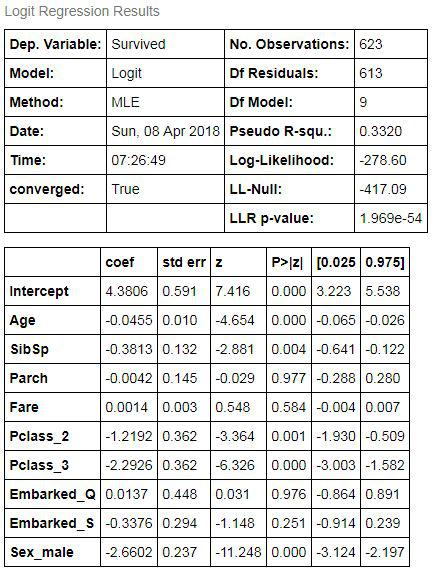
This is the same summary that would be generated in R using the logit function.

Predicting Values on the Test Dataset

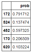
We will now predict the values on the test dataset using the model. Note that the resulting predictive values will be the probability of survival. In order to convert this to binary values, we will round off these values to 0 and 1. We will set a threshold of 0.5 where any value less than 0.5 will be assigned 0 and any value greater than 0.5 will be 1. We now predict the values using the predict command.

Predict = results.predict(test_set)

Converting to a Data Frame

As the above results are in the form of an array, we will be converting them to a data frame and then use the round function to round off the value.

Predict1 = pd.DataFrame(Predict,columns=['prob'])
Predict1.head()

Round Off the Value Using np.round

We will round off these values as we want the predicted values in terms of 1s and 0s. This way we will convert values greater than 0.5 to 1 and values less than 0.5 to 0.

Predict2 = np.round(Predict1['prob'],0)
Predict2.head()

Dataframe for Comparison

Now we will be making a data frame of actual values and predicted values for comparison.

log_test_pred = pd.DataFrame({'actual':test_set['Survived'],'predicted':Predict2})
log_test_pred['predicted']= log_test_pred['predicted'].astype(int)
log_test_pred.head()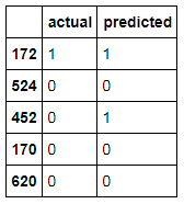

Confusion Matrix

In order to calculate the accuracy of our model, we will be using the metrics package. This package will give you all types of measures such as confusion matrix, accuracy score, area under curve etc. First, we will compute the confusion matrix.

from sklearn import metrics
cm = metrics.confusion_matrix(log_test_pred.actual,log_test_pred.predicted,[0,1])
cm

Accuracy Score

We now calculate the accuracy using the accuracy_score command.

accuracy=metrics.accuracy_score(log_test_pred.actual,log_test_pred.predicted)
accuracy

Our model is 78% accurate however as discussed in the Evaluation of Classification Models under the Theory Section, these methods are insufficient and we require more advanced methods of evaluating our model whose application in Python is discussed in Model Evaluation in Python.

Also, note that logistic regression can be performed by using two packages in Python. One is through the statsmodels and the other package is Scikit-Learn. The statsmodel package deploys simple logistic regression method while Scikit-Learn estimator - LogisticRegression - imposes penalty while training the model. The penalty regularizes the logistic regression model. The penalty can be 'L1' for Lasso and 'L2' for Ridge.

Regularized Logistic Regression

Regularized Logistic Regression can be of two types - Ridge and Lasso. Refer to Regularized Regression Algorithms under the Theory Section to understand the difference between the two. While building models for these in Python, we use penalty='l1' for Lasso and penalty='l2' for Ridge classification. By default, logistic regression takes penalty='l2' as a parameter. A third type is Elastic Net Regularization which is a combination of both penalties l1 and l2 (Lasso and Ridge).

Note that splitting method for statsmodel and Scikit-Learn estimator models is different. Therefore, for all the models to follow Regularized Logistic Regression, we will be using a different method to split the dataset into train and test which will be based on the variables (Features and Target Variable). However, before we split the dataset into train and test components we first need to scale the data.

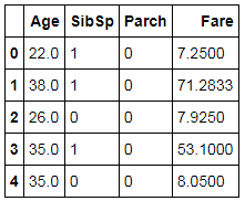
Import StandardScaler to Standardize the Dataset

We will have to first scale the data as Regularized Logistic Regression penalizes the coefficients and hence we cannot have the variables with different scales of measurement. Various models of classification require scaling of data, such as Regularized Logistic Regression (Lasso and Ridge), KNN, SVM and ANN. (We will be using the same scaled dataset for KNN and SVM to predict the survival rate of the passengers.) We first use the dataset TitanicD1 which we had created earlier that has the dummy variables. From there we first extract the numerical variables and apply scaling on them. As there are only two continuous variables in our dataset namely Age and Fare, we will only extract and scale them.

from sklearn.preprocessing import StandardScaler
TitanicD1_feat = TitanicD1[['Age','SibSp','Parch','Fare']]
TitanicD1_feat.head()

We now apply scaling on these numerical features.

scaler = StandardScaler()
scaled = scaler.fit_transform(TitanicD1_feat)
scaled

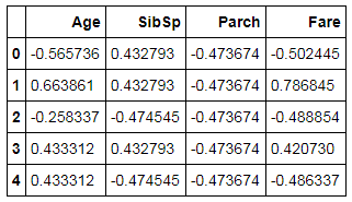
We convert the above output which is an array format into a data frame.

scaled_X = pd.DataFrame(scaled,columns=['Age','SibSp','Parch','Fare'])
scaled_X.head()

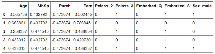
In this step, we concatenate the scaled variables with the leftover dataset (categorical variables).

Titanic_cat = TitanicD1[['Pclass_2','Pclass_3','Embarked_Q','Embarked_S','Sex_male']]
scaled_final = pd.concat([scaled_X,Titanic_cat],axis=1)
scaled_final.head()

Show full table ▾

Splitting Dataset into Train and Test

Here we split the dataset, not in the way we did in Logistic Regression. The method of splitting dataset shown above under the 'Importing Libraries and Preparing Dataset' will be used where we use the train_test_split function to split the dataset into Train and Test.

X1_train,X1_test,Y1_train,Y1_test=train_test_split(scaled_final,TitanicD1['Survived'],test_size=0.3,random_state=123)

Note that the above datasets will be used again when we will be dealing with KNN, SVM and ANN.

Lasso

Import Library

Here instead of statsmodel, we use sklearn and import LogisticRegression as this function provides us with the option of declaring penalties.

from sklearn.linear_model import LogisticRegression

Build Model

We build a Lasso Logistic Regression Model which uses penalty='l1'.

model_lasso = LogisticRegression(penalty='l1')

Fit Model

We now fit the model on the train dataset.

model_lasso.fit(X1_train,Y1_train)

Prediction

In this step, we predict the dependent variable of the test dataset.

pred_lasso = model_lasso.predict(X1_test)

Calculate Accuracy

We import metrics and calculate the accuracy to see how better has a Lasso Logistic Regression fared compared to a simple Logistic Regression Model.

from sklearn import metrics
metrics.accuracy_score(Y1_test,pred_lasso)

The accuracy of this model comes out to be at 80% which is higher than what the simple Logistic Regression using statsmodel provided us where the accuracy was 78%. However, it is again being reminded that this accuracy is not a very valid way of comparing the performance of two models and other methods are explained in the model evaluation blog.

Ridge

Build Model

We build the model for Ridge using penalty='l2'.

model_ridge = LogisticRegression(penalty='l2')
model_ridge.fit(X1_train,Y1_train)

Prediction

We predict the dependent variable of the test dataset.

pred_ridge = model_ridge.predict(X1_test)

Calculate Accuracy

We now calculate the accuracy to compare its results with the simple Logistic and Lasso Logistic Regression models.

metrics.accuracy_score(Y1_test,pred_ridge)

The accuracy provided by Ridge is almost same as Lasso.

Elastic Net

For Regression, we use model ElasticNet whereas for Classification we use Stochastic Gradient Descent Classifier. For classification, we declare loss and penalty. Here, we will define loss equal to log for Logistic Regression and penalty will be equal to elasticnet.

Import Library

Here we use sklearn and import linear_model to use SGD Classifier. We also import warnings to stop any unnecessary warnings when running the model.

import warnings
warnings.filterwarnings("ignore")
from sklearn import linear_model

Initialize Model

In this step we use linear_model.SGDClassifier and initialise the SGD Classifier model using 0.01 as the alpha value.

EN_log = linear_model.SGDClassifier(loss='log',penalty='elasticnet',alpha=0.01)

Fit Model

We now fit the model on the train dataset.

EN_log.fit(X1_train,Y1_train)

Prediction

We predict the dependent variable of the test dataset.

pred_EN_log = EN_log.predict(X1_test)

Calculate Accuracy

We now calculate the accuracy of the SGD Classifier Model.

metrics.accuracy_score(Y1_test,pred_EN_log)

This classifier provides us with 80% accuracy.

Tuning of Parameters

We will now tune the parameters for Regularized Logistic Regression using Grid Search and Random Search. As discussed above, we will first find the model with best parameters and fit the model on the Train dataset. Then, we will predict the values on test dataset and calculate the accuracy score using metrics package. Here we will find the best value of the parameter C which is the inverse of strength of regularization. For Elastic Net, however, we will look for alpha and l1_ratio where l1_ratio is the elasticnet mixer parameter whose value is taken between 0 and 1.

Grid Search - Ridge

We import GridSearchCV from sklearn.model_selection which we will use to tune hyper-parameters.

from sklearn.model_selection import GridSearchCV

Parameters have to be defined first and only then they can be used in the Grid Search. The values of parameters is defined differently in Grid Search and Random Search. Grid Search requires discrete values, whereas Random Search uses a range of the values for parameters.

tuned_parameters = [{'C': [10**-4, 10**-2, 10**0, 10**2, 10**4]}]

We now build the Regularized Logistic Regression model using the Grid Search and fit it on the Train dataset.

model1 = GridSearchCV(LogisticRegression(), tuned_parameters)
model1.fit(X1_train,Y1_train)

The best_params_ command can be used to find the best parameters.

model1.best_params_

In this case, it took C=1 as the best parameter value.

We now predict the Survival on the Test dataset.

pred_model = model1.predict(X1_test)

We compute the accuracy of this model.

metrics.accuracy_score(Y1_test,pred_model)

The accuracy comes out to be at 79%.

Note: Here we have used default penalty which is l2 i.e. Ridge Regression. You can perform the same steps mentioned above for hyperparameter tuning and just add penalty=l1 [LogisticRegression(penalty=l1)]. This will give you results for Lasso.

Grid Search - Elastic Net

For SGD Classifier we will tune two parameters: alpha and l1_ratio.

prams_EN_log = {'alpha' :np.array([1,0.1,0.01,0.001,0.0001]),
         'l1_ratio' :np.array([0.1,0.01,0.001,0.0001,1])}

We now build the SGD Classification model using the Grid Search and fit it on the Train dataset.

EN_log_GS = GridSearchCV(linear_model.SGDClassifier(loss='log',penalty='elasticnet'), param_grid=prams_EN_log)
EN_log_GS.fit(X1_train,Y1_train)

The best_params_ command can be used to find the best parameters.

EN_log_GS.best_params_

We now predict using the EN_log_GS model on the Test dataset.

pred_EN_log_GS = EN_log_GS.predict(X1_test)

We compute the accuracy of this model.

metrics.accuracy_score(Y1_test,pred_EN_log_GS)

The accuracy comes out to be 80%.

Random Search - Ridge

We import RandomizedSearchCV from sklearn.model_selection which will allow us to tune hyper-parameters.

from sklearn.model_selection import RandomizedSearchCV

As the values of C can be in decimals, therefore, we use uniform distribution to define the range of the parameter C. For integers we can use sp_randint, this will take random integer values in a range. In this step, we import uniform from scipy_stats and declare a list of plausible parameters.

from scipy.stats import uniform
C = uniform(0.0001,1)
param_grid = dict(C=C)

We build the model and search for the best parameters. Here we run 100 iterations to come up with the best value of parameter.

model_RS = RandomizedSearchCV(LogisticRegression(), param_distributions=param_grid,n_iter=100)

We now fit the model on the Train dataset.

model_RS.fit(X1_train,Y1_train)

The best_params_ command can be used to find the best parameters.

model_RS.best_params_

The best value of C is considered to be at 0.0945092924075991.

The above model is used to predict the values of the dependent variable in the Test dataset and also the accuracy is calculated.

pred_RS = model_RS.predict(X1_test)
metrics.accuracy_score(Y1_test,pred_RS)

The accuracy comes out to be at 83% which is better than what we got when we used C=1 which was provided by Grid Search.

Note: Here also we have used default penalty which is l2 i.e. Ridge Regression. You can perform hyperparameter tuning for Lasso using Random Search by just declaring penalty=l1 [LogisticRegression(penalty=l1)].

Random Search - Elastic Net

We provide a distribution of values for the 2 hyperparameters.

prams_EN_log_RS = {'alpha' :uniform(0.0001,1),
         'l1_ratio' :uniform(0.0001,1)}

We now build a model using RandomSearchCV and fit it on the Train dataset.

EN_log_RS = RandomizedSearchCV(linear_model.SGDClassifier
(loss='log',penalty='elasticnet'),param_distributions=prams_EN_log_RS,n_iter=100)

EN_log_RS.fit(X1_train,Y1_train)

We use the best_params_ command and check for the best parameters obtained from RandomSearchCV.

EN_log_RS.best_params_

The above model is used to predict the values of the dependent variable in the Test dataset. In this step, we also check for the accuracy obtained by the model.

pred_EN_log_RS = EN_log_RS.predict(X1_test)
metrics.accuracy_score(Y1_test,pred_EN_log_RS)

We get 81% accuracy from the above model.

Decision Tree Classifier

Decision Trees is one of the most commonly used classification algorithms. In very simple words, Decision Trees allow us to come up with flowcharts that are structured as trees and allow us to predict the value of the class variable. Its inner workings have been explained in Decision Trees under the Theory Section.

Splitting Dataset

As we don't require scaling in this case, therefore we will just split our pre-processed dataset TitanicD1 into train and test like we did above. We first start off by separating the dataset with Features and Target variable.

X_T = TitanicD1[['Age', 'SibSp', 'Parch', 'Fare', 'Pclass_2', 'Pclass_3','Embarked_Q', 'Embarked_S', 'Sex_male']]
Y_T = TitanicD1['Survived']

We now split the dataset into Train and Test.

X_train,X_test,Y_train,Y_test=train_test_split(X_T,Y_T,test_size=0.3,random_state=123)

This code makes two train datasets, one with the X variables i.e. Independent Features and one with the Y variable i.e. the Target or Dependent variable.

Importing Libraries

We import tree from sklearn which allows us to create a Decision Tree Classification model.

from sklearn import tree

Initializing Decision Trees Model

Here we initialize the Decision Tree model. Right now we are using no hyperparameters and simply use DecisionTreeClassifier() to initialize.

clf = tree.DecisionTreeClassifier()
clf

Fitting Model

We now fit the above-created model on the Train Dataset.

clf1 = clf.fit(X_train,Y_train)

Prediction and Calculating Accuracy

The Decision Tree model is used to predict the Y variable in the Test dataset. We also check the accuracy of this model on the Test dataset.

Predictions = clf1.predict(X_test)
metrics.accuracy_score(Y_test,Predictions)

The accuracy of this Decision Tree model comes out to be at 79%.

Tree Visualization

We can visualize the above-created Decision Tree. This helps in further understanding how the decision tree algorithm is working.

Install and Import graphviz

We have to install graphviz in Python by typing pip install graphviz in the command window. Once done we can import the graphviz library in Python.

import graphviz

Creating Decision Tree Visualization

We now use graphviz to create the Decision Tree flowchart.

dot_data = tree.export_graphviz(clf1, out_file=None, max_depth=3,
                         feature_names=X_T.columns,
                         class_names=['0','1'],
                         filled=True, rounded=True,
                         special_characters=True)

graph2 = graphviz.Source(dot_data)

Saving Image

To save the tree image in a pdf file, we use the following code.

graph2.render('final')

Opening Saved Image

We import os and use the following code to open the saved pdf file of the tree.

import os
os.startfile('final.pdf')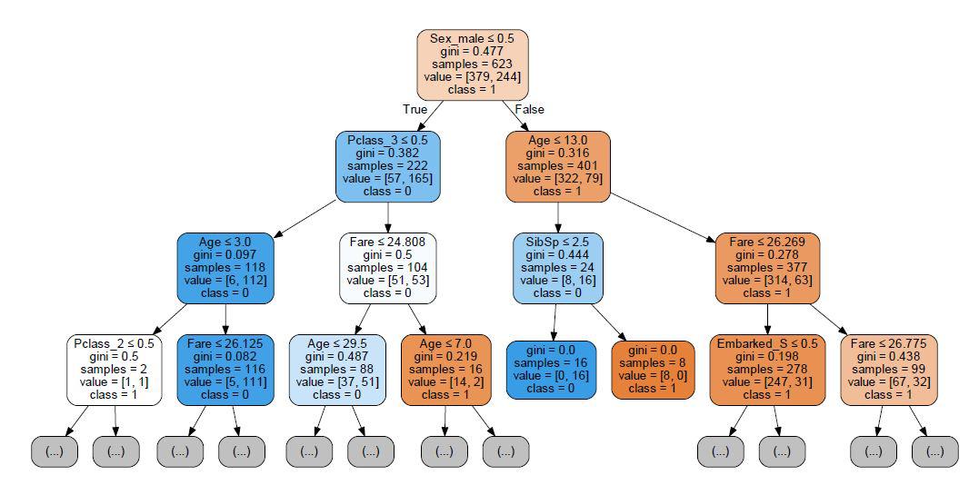

Tuning Hyperparameters

To show an example of how hyperparameters can be tuned, we take the following four parameters for tuning: max_features which is the number of features to be considered for looking for the best split, the minimum sample split, the minimum sample leaf and the max_depth which is the maximum depth of the tree. All such hyperparameters have been explained in the theory section. You may select other parameters also if you want more control over the process and desire more accuracy.

Grid Search

Here we define the plausible values for our four parameters.

params = {'max_features': ['auto', 'sqrt', 'log2'],
       'min_samples_split': [2,3,4,5,6,7,8,9,10],
       'min_samples_leaf':[1,2,3,4,5,6,7,8,9,10,11],
         'max_depth':[2,3,4,5,6,7,8,9]}

We now initialize the Decision Tree model.

DTC = tree.DecisionTreeClassifier()

We now build a model using GridSearchCV and fit it on the Train dataset.

DTC1 = GridSearchCV(DTC, param_grid=params)
DTC1.fit(X_train,Y_train)

The best_params_ command can be used to find the best parameters.

modelF = DTC1.best_estimator_
modelF

The above model with the above-mentioned values of hyperparameters is used to predict the values of the dependent variable in the Test dataset and also the accuracy is calculated.

pred_modelF = modelF.predict(X_test)
metrics.accuracy_score(Y_test,pred_modelF)

The accuracy comes out to be 82%.

Random Search

As mentioned earlier, for defining parameters that are integers we use sp_randint which we import from scipy.stats.

from scipy.stats import randint as sp_randint

param_grid2 = {'max_features': ['auto', 'sqrt', 'log2'],
          'min_samples_split': sp_randint(2,10),
          'min_samples_leaf': sp_randint(1,11),
         'max_depth':sp_randint(2,8)}

We now build a model using RandomSearchCV and fit it on the Train dataset.

DTC_RS = RandomizedSearchCV(DTC, param_distributions=param_grid2,n_iter=100)
DTC_RS1 = DTC_RS.fit(X_train,Y_train)
DTC_RS1

We use the best_params_ command and check for the best parameters obtained from RandomSearchCV.

DTC_RS1.best_params_

The above model with the best parameters is used to predict the values of the dependent variable in the Test dataset and also the accuracy is calculated.

pred_RS_DTC = DTC_RS1.predict(X_test)
metrics.accuracy_score(Y_test,pred_RS_DTC)

The Accuracy comes out to be at 83%.

K Nearest Neighbour

KNN is a distance-based algorithm which predicts value based on the number of class observations found in its neighbourhood. For a detailed understanding of KNN refer to K Nearest Neighbour under the Theory Section.

Importing KNeighborsClassifier Package

To run KNN in Python, we require KNeighborsClassifier which we import from sklearn.neighbors.

from sklearn.neighbors import KNeighborsClassifier

Initializing and Fitting KNN Model

In this step, we first initialize the KNN model. We then fit this model on the Train Dataset. Note that this Train dataset is what we used earlier for Regularized Logistic Regression. For KNN we need to have a standardized dataset as it uses distance as a parameter for its functioning. Therefore, for this model, we use a dataset which has all the numerical observations scaled except the target variable.

knn = KNeighborsClassifier()
knn.fit(X1_train,Y1_train)

Predict and Check Accuracy

The above model is used to predict the values of the dependent variable in the Test dataset and the accuracy is calculated.

pred_knn = knn.predict(X1_test)
metrics.accuracy_score(Y1_test,pred_knn)

The accuracy comes out to be at 80%.

Tuning Hyperparameters

In this blog post, we will tune four hyperparameters for KNN: n_neighbours where we declare the different number of Neighbours that can be considered, algorithm where we can use methods such as K-D trees which help in speeding up the testing phase, leaf_size which helps the algorithm in deciding when to switch from usual brute force method to tree-based methods such as K-D trees and weights where alternatives to majority voting can be provided. (All such hyperparameters have been explained in the theoretical explanation of KNN to which one can refer for more information. Also, there are a lot of other hyperparameters to choose from which you may select if you want more control over the process and desire more accuracy.)

Grid Search

We define the values for our four parameters.

params_knn = {'n_neighbors':[5,6,7,8,9,10,12],
          'leaf_size':[1,2,3,5],
          'weights':['uniform', 'distance'],
          'algorithm':['auto', 'ball_tree','kd_tree','brute']}

We now build a KNN model using GridSearchCV and fit it on the Train dataset.

model_knn_GS = GridSearchCV(KNeighborsClassifier(), param_grid=params_knn)
model_knn_GS.fit(X1_train,Y1_train)

We use best_params_ to check for the best parameters.

model_knn_GS.best_params_

The above model with the above-mentioned values of hyperparameters is used to predict the values of the dependent variable in the Test dataset and also the accuracy is calculated.

pred_knn_GS = model_knn_GS.predict(X1_test)
metrics.accuracy_score(Y1_test,pred_knn_GS)

The accuracy obtained from this model is 82%.

Random Search

We define a range of values for our four parameters.

params_knn_rs = {'n_neighbors':sp_randint(5,12),
          'leaf_size':sp_randint(1,5),
          'weights':['uniform', 'distance'],
          'algorithm':['auto', 'ball_tree','kd_tree','brute']}

We now build a KNN model using RandomSearchCV and fit it on the Train dataset.

KNN_RS = RandomizedSearchCV(KNeighborsClassifier(), param_distributions=params_knn_rs,n_iter=250)
KNN_RS.fit(X1_train,Y1_train)

We now check for the best parameters obtained using Random Search.

KNN_RS.best_params_

We use the above model and the best combination of hyperparameters and predict the values of the dependent variable in the Test dataset and also the accuracy is calculated.

pred_knn_rs = KNN_RS.predict(X1_test)
metrics.accuracy_score(Y1_test,pred_knn_rs)

The accuracy comes out to be around 81%.

Support Vector Machine

SVM is a technique commonly used for solving classification problems. It has been explained in the Support Vector Machines under the Theory Section. Here we will put it to use using Python.

Importing SVC Package

To run SVM in Python, we require SVC which we import from sklearn.svm.

from sklearn.svm import SVC

Initializing and Fitting Model

In this step, we initialize the SVM model and fit it on the Train dataset. Note that SVM requires a standardized dataset to fit the model and make predictions and we will use the dataset that we have used earlier where the numerical features have been scaled and dummy variables have been created for categorical features.

model_SVM = SVC()
model_SVM.fit(X1_train,Y1_train)

Predict and Check Accuracy

The above model is used to predict the values of the dependent variable in the Test dataset and the accuracy is calculated.

pred_svm = model_SVM.predict(X1_test)
metrics.accuracy_score(Y1_test,pred_svm)

The accuracy got from the SVM model is 83% which is the highest value of accuracy we have got so far.

Tuning Hyperparameters

In this blog post, we will tune two hyperparameters for SVM which are the value of C and the type of kernel.

Grid Search

We define the plausible values for our two parameters.

params_SVM = {'C': [0.01,0.1,1],
          'kernel': ['linear','rbf']}

We now build an SVM model using GridSearchCV and fit it on the Train dataset.

model_svm_GS = GridSearchCV(SVC(), param_grid=params_SVM)
model_svm_GS.fit(X1_train,Y1_train)

We now check the selected best parameters.

model_svm_GS.best_params_

The above model and hyperparameters are used to predict the values of the dependent variable in the Test dataset and calculate the accuracy.

pred_svm_GS = model_svm_GS.predict(X1_test)
metrics.accuracy_score(Y1_test,pred_svm_GS)

The accuracy obtained from this model is 83%.

Random Search

We give a range of values for our two parameters.

params_RS1 = {'C': uniform(0.01,1),
          'kernel': ['linear','rbf']}

We now build an SVM model using RandomSearchCV and fit it on the Train dataset.

SVM_RS = RandomizedSearchCV(SVC(),param_distributions=params_RS1,n_iter=100)
SVM_RS.fit(X1_train,Y1_train)

We now check for the best parameters obtained using Random Search.

SVM_RS.best_params_

We use the above SVM model and the best combination of hyperparameters and predict the values of the dependent variable in the Test dataset and also the accuracy is calculated.

pred_svm_rs= SVM_RS.predict(X1_test)
metrics.accuracy_score(Y1_test,pred_svm_rs)

The accuracy comes out to be 83%.

Artificial Neural Networks

Artificial Neural Networks have been explained in detail in the Theory Section and here we will be creating an ANN model on the Titanic dataset.

Importing Library

To create an ANN model in Python, we can choose from various libraries. Tensorflow is among the most famous library often used to create deep learning models. Another famous library is Keras which is more user-friendly when compared to Tensorflow. In this blog post, however, we will be using a very basic library for creating an ANN Model, known as the MLPClassifier.

from sklearn.neural_network import MLPClassifier

Initializing and Fitting Model

In this step, we initialise the ANN model and fit it on the Train dataset. Note that ANN requires a standardized dataset to fit the model and make predictions and we will use the dataset that we have used earlier where the numerical features have been scaled and dummy variables have been created for categorical features.

ann = MLPClassifier()
ann.fit(X1_train,Y1_train)

Predict and Check Accuracy

The above model is used to predict the values of the dependent variable in the Test dataset and along with this, the accuracy is also calculated.

pred_ann = ann.predict(X1_test)
metrics.accuracy_score(Y1_test,pred_ann)

The accuracy got from the ANN model is 82%.

Tuning Hyperparameters

In this blog post, we will tune a couple of hyperparameters. Here we can tune the activation function of the hidden layers. learning_rate_init parameter is used to increase accuracy as slower the learning rate, better is the accuracy. We can also tune the batch size and warm_start for better results.

Grid Search

Here we define the above mentioned four parameters.

params_ann = {'activation': ['identity', 'logistic', 'tanh', 'relu'],
          'batch_size': [10,15,25,32,40,50],
          'learning_rate_init':[0.05,0.1,0.2],
          'warm_start':['True','False']}

We now initialize the MLP Classifier model.

ann_grid = GridSearchCV(MLPClassifier(), param_grid=params_ann)

We now fit the model on the Train dataset.

ann_grid.fit(X1_train,Y1_train)

The best_params_ command can be used to find the best parameters.

ann_grid.best_params_

The above model with the above-mentioned values of hyperparameters is used to predict the values of the dependent variable in the Test dataset and also the accuracy is calculated.

ann_pred1 = ann_grid.predict(X1_test)
metrics.accuracy_score(Y1_test,ann_pred1)

The accuracy comes out to be 83%.

Random Search

We define the range of our four parameters.

params_ann_RS = {'activation': ['identity', 'logistic', 'tanh', 'relu'],
          'batch_size': sp_randint(10,50),
          'learning_rate_init':uniform(0.05,0.2),
          'warm_start':['True','False']}

We now build a model using RandomSearchCV and fit it on the Train dataset.

ANN_RS = RandomizedSearchCV(MLPClassifier(), param_distributions=params_ann_RS,n_iter=100)
ANN_RS.fit(X1_train,Y1_train)

We use the best_params_ command and check for the best parameters obtained from RandomSearchCV.

ANN_RS.best_params_

The above model with the best parameters is used to predict the values of the dependent variable in the Test dataset and also the accuracy is calculated.

ann_pred_RS = ANN_RS.predict(X1_test)
metrics.accuracy_score(Y1_test,ann_pred_RS)

The Accuracy comes out to be at 83%.

Naive Bayes

Naive Bayes is a probabilistic model which uses the Bayesian Theorem for its working. It has been explored under the Theory Section in the blog Naive Bayes. In this blog, we will use Naive Bayes to solve this classification problem of who survives and who doesn't.

Importing GaussianNB Package

To run a Naive Bayes model in Python, we require GaussianNB which we import from sklearn.naive_bayes.

from sklearn.naive_bayes import GaussianNB

Initializing and Fitting Model

In this step, we initialise the Naive Bayes model and fit it on the Train dataset.

NB = GaussianNB()
NB.fit(X_train,Y_train)

Predict and Check Accuracy

The above model is used to predict the values of the dependent variable in the Test dataset and calculate the accuracy.

pred_NB = NB.predict(X_test)
metrics.accuracy_score(Y_test,pred_NB)

The accuracy got from the Naive Bayes model is 82%.

Ensemble Models

Ensemble models are used to improve the predictive performance of a model. Ensemble methods have been discussed in Ensemble Methods under the Theory Section. In this blog, we will use four main Ensemble methods to create classification models to predict the survival of passengers on the Titanic. These are Bagging, Random Forest, AdaBoosting, Gradient Boosting and XgBoost. We will also be using the Stacking technique for Ensemble Classification in Python.

Bagging Classifier

Bagging (Bootstrap Aggregating) involves fitting multiple models on different subsets of the training dataset, then combining the predictions from all models. Bagging is used to reduce variance of a decision tree. This technique is applicable to other classification methods however mostly it is used with Decision Trees. When applied to decision trees, this approach is commonly known as bagged decision trees.

Importing BaggingClassifier Package

To run the Bagging Classifier, we import BaggingClassifier from sklearn.ensemble.

from sklearn.ensemble import BaggingClassifier

Initializing and Fitting Model

In this step, we initialize the Bagging Classifier model and fit it on the Train dataset.

Bag = BaggingClassifier()
Bag.fit(X_train,Y_train)

Predict and Check Accuracy

We use the above model to predict the values of the dependent variable in the Test dataset and calculate the accuracy.

pred_Bag = Bag.predict(X_test)
metrics.accuracy_score(Y_test,pred_Bag)

The accuracy got from this Bagging Classifier is 83%.

Tuning Hyperparameters

We will now tune the parameters using Grid Search and Random Search for the Bagging Classifier. In this blog post, we will tune two hyperparameters namely max_samples which is the fraction of the dataset used to build each learner and max_features which is the number of features used for each base learner.

Grid Search

params_Bag = {'max_samples': [0.5,1.0],
          'max_features': [0.5,1.0]}

Bag_GS = GridSearchCV(BaggingClassifier(), param_grid=params_Bag)
Bag_GS.fit(X_train,Y_train)

Bag_GS.best_params_

pred_Bag_GS = Bag_GS.predict(X_test)
metrics.accuracy_score(Y_test,pred_Bag_GS)

The accuracy comes out to be 82%.

Random Search

params_Bag_RS = {'max_samples': uniform(0.5,1.0),
          'max_features': uniform(0.5,1.0)}

Bag_RS = RandomizedSearchCV(BaggingClassifier(), param_distributions=params_Bag_RS,n_iter=100)
Bag_RS.fit(X_train,Y_train)

Bag_RS.best_params_

pred_Bag_RS = Bag_RS.predict(X_test)
metrics.accuracy_score(Y_test,pred_Bag_RS)

The accuracy comes out to be at 83%.

Random Forest Classifier

Random Forest is an ensemble algorithm which uses multiple Decision Trees to get results. It is based on the Bagging method. To understand the algorithm behind it, refer to Random Forests under the Theory Section.

Importing RandomForestClassifier Package

To run the Random Forest Classifier, we import RandomForestClassifier from sklearn.ensemble.

from sklearn.ensemble import RandomForestClassifier

Initializing and Fitting Model

In this step, we initialize the Random Forest Classifier model and fit it on the Train dataset.

RF = RandomForestClassifier()
RF.fit(X_train,Y_train)

Predict and Check Accuracy

pred_RF = RF.predict(X_test)
metrics.accuracy_score(Y_test,pred_RF)

The accuracy got from this Random Forest model is 84%.

Tuning Hyperparameters

Grid Search

params_RF = {'max_features': ['auto', 'sqrt', 'log2'],
          'min_samples_split': [2,3,4,5,6,7,8,9,10],
          'min_samples_leaf': [1,2,3,4,5,6,7,8,9,10,11],
          'max_depth':[2,3,4,5,6,7,8,9]}

RF_GS = GridSearchCV(RandomForestClassifier(), param_grid=params_RF)
RF_GS.fit(X_train,Y_train)

RF_GS.best_params_

pred_RF_GS = RF_GS.predict(X_test)
metrics.accuracy_score(Y_test,pred_RF_GS)

The accuracy comes out to be at 83%.

Random Search

params_RF_RS = {'max_features': ['auto', 'sqrt', 'log2'],
          'min_samples_split': sp_randint(2,10),
          'min_samples_leaf': sp_randint(1,11),
          'max_depth':sp_randint(2,8)}

RF_RS = RandomizedSearchCV(RandomForestClassifier(), param_distributions=params_RF_RS,n_iter=100)
RF_RS.fit(X_train,Y_train)

RF_RS.best_params_

pred_RF_RS = RF_RS.predict(X_test)
metrics.accuracy_score(Y_test,pred_RF_RS)

The accuracy comes out to be at 83%.

AdaBoost Classifier

AdaBoost or Adaptive Boosting is a method used to improve the performance of classification models. In simple terms, AdaBoost works by fitting a model and then modifying the weights of the correct and incorrect predictions by the model. Weights are increased for cases that are more difficult to classify and decreased for cases that are easy to classify. Subsequent classifiers therefore are required to focus primarily on those difficult cases. It has been explained in detail in Ensemble Methods under the Theory Section.

Importing AdaBoostClassifier Package

from sklearn.ensemble import AdaBoostClassifier

Initializing and Fitting Model

AB = AdaBoostClassifier()
AB.fit(X_train,Y_train)

Predict and Check Accuracy

pred_AB = AB.predict(X_test)
metrics.accuracy_score(Y_test,pred_AB)

The accuracy got from this AdaBoosting model is 84%.

Tuning Hyperparameters

Grid Search

params_AB = {'n_estimators': [1,10,20,50,100,200],
          'learning_rate': [0.01,0.1,0.2,0.3,1.0]}

AB_GS = GridSearchCV(AdaBoostClassifier(), param_grid=params_AB)
AB_GS.fit(X_train,Y_train)
AB_GS.best_params_

pred_AB_GS = AB_GS.predict(X_test)
metrics.accuracy_score(Y_test,pred_AB_GS)

The accuracy comes out to be at 83%.

Random Search

params_AB_RS = {'n_estimators': sp_randint(1,100),
          'learning_rate': uniform(0.01,1.0)}

AB_RS = RandomizedSearchCV(AdaBoostClassifier(), param_distributions=params_AB_RS,n_iter=100)
AB_RS.fit(X_train,Y_train)
AB_RS.best_params_

pred_AB_RS = AB_RS.predict(X_test)
metrics.accuracy_score(Y_test,pred_AB_RS)

The accuracy comes out to be at 83%.

Gradient Boosting Classifier

Gradient Boosting is another method of Boosting which is used to improve the performance of classification models. It uses a Gradient Descent method while iterating over the trees. It has been explained in detail in Ensemble Methods under the Theory Section.

Importing GradientBoostingClassifier Package

from sklearn.ensemble import GradientBoostingClassifier

Initializing and Fitting Model

GB = GradientBoostingClassifier()
GB.fit(X_train,Y_train)

Predict and Check Accuracy

pred_GB = GB.predict(X_test)
metrics.accuracy_score(Y_test,pred_GB)

The accuracy got from this Gradient Boosting model is 82%.

Tuning Hyperparameters

Grid Search

params_GB = {'n_estimators': [1,10,20,50,100,200],
          'max_depth': [2,3,4,5,6,7,8,9],
          'learning_rate': [0.01,0.1,0.2,0.3,1.0]}

GB_GS = GridSearchCV(GradientBoostingClassifier(), param_grid=params_GB)
GB_GS.fit(X_train,Y_train)
GB_GS.best_params_

pred_GB_GS = GB_GS.predict(X_test)
metrics.accuracy_score(Y_test,pred_GB_GS)

The accuracy comes out to be at 82%.

Random Search

params_GB_RS = {'n_estimators': sp_randint(1,100),
          'max_depth': sp_randint(2,8),
          'learning_rate': uniform(0.01,1.0)}

GB_RS = RandomizedSearchCV(GradientBoostingClassifier(), param_distributions=params_GB_RS,n_iter=100)
GB_RS.fit(X_train,Y_train)
GB_RS.best_params_

pred_GB_RS = GB_RS.predict(X_test)
metrics.accuracy_score(Y_test,pred_GB_RS)

The accuracy comes out to be at 83%.

XGBoost Classifier

XGBoost or Extreme Gradient Boosting is a well-known library used to build classification models. In recent years it has become one of the most popular and widely used algorithms for modeling. It is highly efficient and uses a regularization technique to prevent overfitting of models.

Installing XGBoost

We will have to first install XGBoost by typing pip install xgboost in the command prompt.

Importing XGBClassifier Package

from xgboost import XGBClassifier

Initializing and Fitting Model

XGB = XGBClassifier()
XGB.fit(X_train,Y_train)

Predict and Check Accuracy

pred_XGB = XGB.predict(X_test)
metrics.accuracy_score(Y_test,pred_XGB)

The accuracy got from this XGBoost model is 83%.

Tuning Hyperparameters

Grid Search

params_XGB = {'n_estimators': [1,10,20,50,100,200],
          'max_depth': [2,3,4,5,6,7,8,9],
          'learning_rate': [0.01,0.1,0.2,0.3,1.0]}

XGB_GS = GridSearchCV(XGBClassifier(), param_grid=params_XGB)
XGB_GS.fit(X_train,Y_train)
XGB_GS.best_params_

pred_XGB_GS = XGB_GS.predict(X_test)
metrics.accuracy_score(Y_test,pred_XGB_GS)

The accuracy comes out to be at 83%.

Random Search

params_XGB_RS = {'n_estimators': sp_randint(1,100),
          'max_depth': sp_randint(2,8),
          'learning_rate': uniform(0.01,1.0)}

XGB_RS = RandomizedSearchCV(XGBClassifier(), param_distributions=params_XGB_RS,n_iter=100)
XGB_RS.fit(X_train,Y_train)
XGB_RS.best_params_

pred_XGB_RS = XGB_RS.predict(X_test)
metrics.accuracy_score(Y_test,pred_XGB_RS)

The accuracy comes out to be at 82%.

Stacking

Stacking is an Ensemble Learning technique that combines multiple classification or regression models via a meta-classifier or a meta-regressor. To understand how Stacking works, one can refer to the Ensemble Methods blog under the Theory Section. Here we will be creating Stacking models using the StackingClassifier package from mlxtend.

Installing mlxtend

We have to first install mlxtend by typing pip install mlxtend in the command prompt.

Importing Packages

Here we import the Logistic Regression, Decision Tree, KNN and SVM Classifiers from sklearn to use as our base classifiers. We also import the StackingClassifier.

from sklearn.linear_model import LogisticRegression
from sklearn.tree import DecisionTreeClassifier
from sklearn.neighbors import KNeighborsClassifier
from sklearn.svm import SVC
from mlxtend.classifier import StackingClassifier

Defining Base Classifiers

We now define the base classifiers and the meta-classifier for our Stacking model.

clf1 = KNeighborsClassifier(n_neighbors=1)
clf2 = DecisionTreeClassifier()
clf3 = SVC()
lr = LogisticRegression()

Initializing the Stacking Model

We now initialize the Stacking Classifier with our base and meta-classifiers.

sclf = StackingClassifier(classifiers=[clf1,clf2,clf3],
                           meta_classifier=lr)

Fitting the Model

We now fit the Stacking model on the Train dataset.

sclf.fit(X_train,Y_train)

Predicting and Calculating Accuracy

We now predict the values of the dependent variable in the Test dataset and calculate the accuracy of the Stacking model.

stack_pred = sclf.predict(X_test)

from sklearn import metrics
metrics.accuracy_score(Y_test,stack_pred)

The accuracy from the Stacking model comes out to be at 82%.