// application · python

Inferential Statistics in Python

Inferential statistics are used to draw inferences from the sample of a huge data set. Random samples of data are taken from a population, which is then used to describe and make inferences and predictions about the population. In the Theory section, various Inferential Statistics were explored and in this blog, all those inferential statistics will be put to use using Python.

In this section, the following topics will be explored:

• Z Scores & Z-Test
• t-Tests
• F-test
• Correlation Coefficients
• Chi-Square

Preliminary Libraries

Note that certain preliminary libraries are to be imported in Python to work on arrays and data frames for statistical analysis.

To do so, we first will import the preliminary libraries such as numpy and pandas. Both these are very important packages where Numpy is used for operations on arrays whereas pandas is used for performing various operations on DataFrames.

import numpy as np
import pandas as pd
import scipy.stats

Z Scores, Z-Test

Z-Scores are used to calculate the probability of a score occurring within our normal distribution. This helps us to compare scores of two or more different normal distributions.

Z Value

Import Dataset: We import a hypothetical data set having exam scores of students.

Z_ScoresData = pd.read_excel("C:/Users/user/Desktop/Data Sets/Marks_Scored.xls")
Z_ScoresData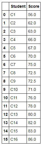

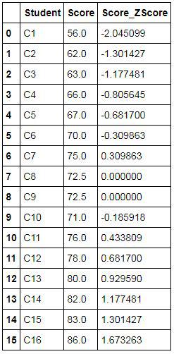
Show full table ▾

Calculating Z Score

The following code can be used to compute Z scores. Here we compute the Z Score for the 'Score' column in the Z-Score dataset. Here we use a function called ddof which is used to modify the divisor sum of the squares of the samples-mean. Divisor is N-ddof. By default, ddof is 0. For sample std, you can put ddof=1.

Z_ScoresData['Score_ZScore'] = (Z_ScoresData['Score'] - Z_ScoresData['Score'].mean())/Z_ScoresData['Score'].std(ddof=0)
Z_ScoresData

Show full table ▾

Exporting Results

The above output can be exported to an excel file using the following command. Here we are exporting the output to a folder in xls format.

Z_ScoresData.to_excel("C:/Users/user/Desktop/Data Sets/Z_ScoresData.xls")

Finding Percentage / Area Under the Curve

We can find out the percentage of people who scored above 70. We take the mean and standard deviation to calculate the area under the curve. Here we use the following code for finding the area under the curve, to find the percentage of students who scored more than 70 marks. 8.06807 is std and 72.5 is mean.

cutOffPoint = 70
print(1-(scipy.stats.norm(72.5, 8.06807).cdf(70)))

Z-Test

Z-test is used to test whether the two datasets are similar or not.

Import Dataset: We take a population dataset and a random sample of the population dataset. We first import the population dataset.

HeightDataPop = pd.read_csv("C:/Users/user/Desktop/Data Sets/Heightof200ppl.csv")

We now import a dataset which is a random sample of the above dataset, i.e. a sample.

HeightDataSample = pd.read_excel("C:/Users/user/Desktop/Data Sets/HeightDataSample.xls")

Comparing Mean: We calculate the population mean.

Mean1 = HeightDataPop['Height (in cm)'].mean()
Mean1

We also calculate the mean of this sample (sample mean).

Mean2 = HeightDataSample['Height(in cm)'].mean()
Mean2

We find that the mean of the population (164.075) and its sample (162.23076923076923) is different, however as we know that the sample is a part of the population only, the results of our Z-Test should indicate that the difference between their mean is statistically insignificant, especially if the sample size is more than 30. To confirm this we perform a Z-Test.

Converting the concerned variable into an array: We extract the 'Height(in cm)' variable from both the population and the sample dataset and convert it into an array for ease of working. We first start off by converting the variable from the population.

X2 = np.array(HeightDataPop['Height (in cm)'])

We also convert the variable in the sample dataset into an array and in the output, we can see that we have more than 30 observations.

Y2 = np.array(HeightDataSample['Height(in cm)'])
Y2

Import the package for performing Z Test: From the package statsmodels.stats.weightstats we import ztest to perform the required statistics.

from statsmodels.stats.weightstats import ztest

Run Z Test: We can now run a Z Test using the function ztest, where we input the two arrays and provide the population mean.

ztest(Y2,x2=None,value=Mean1)

In the output, we get the Z Statistic to be at -1.190425246505336 while the p-value comes out to be 0.2338792950232519. As discussed in Z scores, Z test and Probability Distribution, our null hypothesis in this scenario will be that both the datasets are significantly similar. If we consider the significance level to be at 5%, then to accept the null hypothesis, our p-value should be more than the chosen significance level. In our example, the p-value is well above 0.05 (5%), thus the Z-Test correctly indicates that the means of both the datasets are the same and are not statistically significantly different from each other.

t-Test

t-Test is used to see whether two groups are similar or not. Z-test is also used for the same purpose, however, the difference between these tests is that the Z-test is used when the sample size is greater than 30, whereas t-Test is used when the sample size is less than 30. The difference has been explored in Brief Intro to T Test. There are different types of t-Tests for different scenarios and we put them to use below.

Two-sided One-Sample t-Test

Import the package for performing various t-Test: We import scipy.stats to perform the various t-Tests.

import scipy.stats as stats

Import Dataset: We will be working on a hypothetical Diamond dataset which has the information of the diamonds that were sold in a shop.

DiamondData = pd.read_excel("C:/Users/user/Desktop/Data Sets/DiamondData.xls")
DiamondData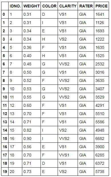

Show full table ▾

Mean of the concerned variable: We will be using the 'WEIGHT' variable to find if the value of 0.5 is statistically greater or lower than the mean of it or not. We first calculate the mean of this variable.

DiamondData['WEIGHT'].mean()

We find that the mean of the variable 'WEIGHT' is 0.5535 which is greater than 0.5, however, we need to run a t-Test to find if the difference is statistically significant or not.

Perform Two-Tailed t-Test: We perform a One-Sample t-Test where we try to find whether the mean of the variable 'WEIGHT' is statistically greater than 0.5 or not. Since this is a two-sided one-sample t-test, our Null Hypothesis is that the mean of 'WEIGHT' equals 0.5, and the Alternative Hypothesis is that it is not equal to 0.5. We now run a One-Sample t-Test to test this hypothesis.

stats.ttest_1samp(DiamondData['WEIGHT'],0.5)

Our p-value comes out to be 0.19297392861206744 which is greater than 0.05 (5% significance level), therefore, we fail to reject the null hypothesis that the mean equals 0.5; the difference from 0.5 is not statistically significant.

Independent t-Test

Import Dataset: Here we import an arbitrary, hypothetical dataset with patient ID, age and gender as variables.

AgeData = pd.read_csv("C:/Users/user/Desktop/Data Sets/data1.csv")
AgeData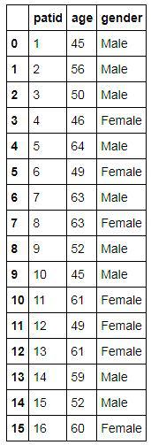

Show full table ▾

Extracting a combination of observations: In this example, we intend to compare the age of Male and Female patients and see if the difference between their age is statistically significant or not. To do so we first extract the age of Male and Female patients separately.

Female_Age = AgeData[AgeData['gender'] == 'Female']['age']
Male_Age = AgeData[AgeData['gender'] == 'Male']['age']

Comparing Mean: We calculate the mean age of both the male and female patients to see if it is different or not. We first calculate the mean age of the Female patients.

Female_Age.mean()

We also calculate the mean age of the male patients.

Male_Age.mean()

We find that the mean age of female patients (55.57142857142857) is different from the mean age of the male patients (54.0). However, we need to perform an Independent t-Test to find if the difference is statistically significant or not.

Running Independent t-Test: We run an Independent t-Test using the function stats.ttest_ind.

stats.ttest_ind(a=Female_Age,b=Male_Age,equal_var=False)

Our null hypothesis is that both groups are statistically significantly similar. Here, the p-value is greater than 0.05, therefore, we accept the null hypothesis that these two groups are significantly similar. Even though the sample means differ, the difference between them is not statistically significant and can be attributed to sampling error.

Paired t-Test

Import Dataset: We import a hypothetical dataset that has marks of students in two different tests. Here we presume that they are the same tests undertaken over a period of time.

ScoresData = pd.read_excel("C:/Users/user/Desktop/Data Sets/Student Test Scores.xls")
ScoresData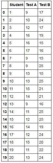

Show full table ▾

Extracting Variables: We extract the scores of both the tests. Here Test A is presumed as the test scores taken before a certain teaching program and the scores in Test B are supposedly the marks of the students on the same tests taken after the program.

before = ScoresData['Test A']
after = ScoresData['Test B']

Running Paired t-Test: We need to find whether the marks/score of the students have changed over time or not. For this, we compare the mean of the two tests and see if they are statistically significantly different from each other or not. Here our null hypothesis is that both test scores are significantly similar.

stats.ttest_rel(a = before, b= after)

We find that the p-value comes out to be 1.2167687282184405e-06 which is very much less than 0.05 (significance level of 5%). Therefore, we reject the null hypothesis, i.e. these test scores are significantly different from each other.

F-test

Different types of F-Tests have been discussed under the theoretical blog for F-Tests, however, the most common F test is One-Way ANOVA. We can use the Age data used in the Independent t-Test and find if the age of males and females is statistically significantly different from each other or not. For this, we run a One-Way ANOVA using a function called stats.f_oneway.

stats.f_oneway(Female_Age,Male_Age)

Correlation Coefficients

Import Dataset: To come up with correlation coefficients, we use the diamond dataset that we have used above for performing the Two-Tailed t-Test.

DiamondData = pd.read_excel("C:/Users/user/Desktop/Data Sets/DiamondData.xls")
DiamondData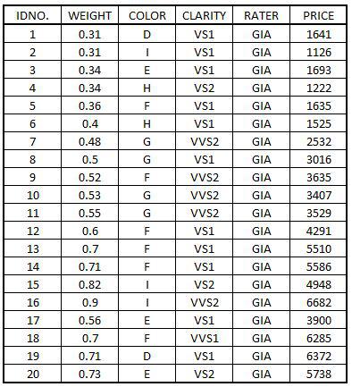

Show full table ▾

Import Packages: When using Correlation Coefficients, scatterplots are extensively used and for this we import matplotlib. We also run a command %matplotlib inline so that the graphs are not displayed separately on a window.

import matplotlib
%matplotlib inline

Scatter Plot

We create a scatterplot to study the correlation between two variables. In this example we chose two variables, 'WEIGHT' and 'PRICE', from our Diamond dataset.

ScatterPlot = DiamondData.plot(kind='scatter',x='WEIGHT',y='PRICE',figsize=(7,7),title='Scatter Plot - Correlation',fontsize=12)

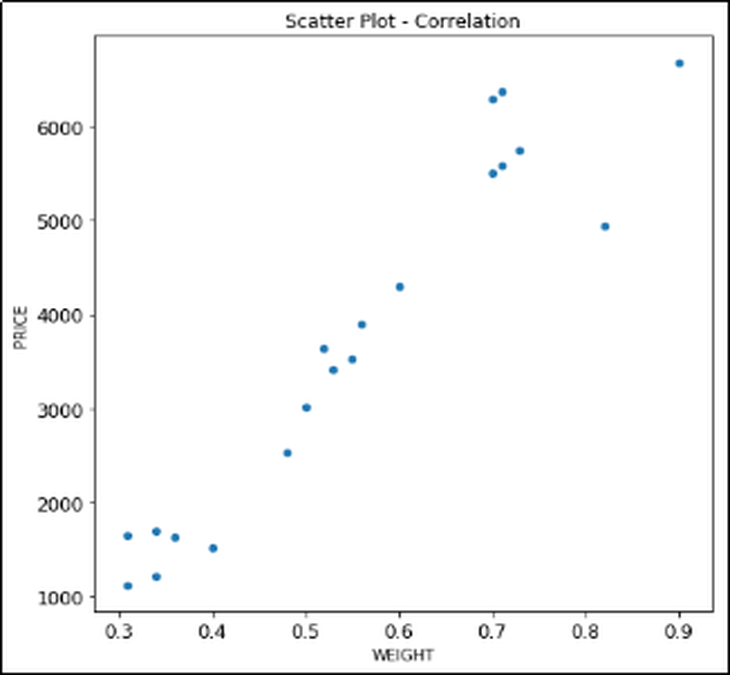
The scatterplot shows a positive correlation between the two variables, and thus there is a direct relation between Price and Weight of the diamond. An increase in weight will correspond to an increase in the Price of that diamond.

Calculating Correlation Coefficient

If we need to properly quantify the relationship between the two variables, then rather than going for a visual approach, we are required to calculate the correlation coefficient. We do this by using a function called corr.

DiamondData['WEIGHT'].corr(DiamondData['PRICE'])

The correlation coefficient comes out to be 0.9541459563876661 which is well above 0 and a lot closer to 1, which shows that a very strong positive correlation exists between the two variables.

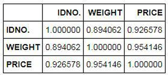
Correlation Coefficient Matrix

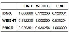
If we have a lot of variables, then rather than calculating the correlation coefficient for each combination of variables, we can come up with a Correlation Coefficient Matrix. Here all the diagonal values will be 1 while the correlation coefficient will be there for all the combinations of the numerical variables. There are two methods of calculating the Correlation Coefficient and its matrix - Pearson and Spearman.

Correlation Coefficient matrix using Pearson:

DiamondData.corr(method='pearson')

Correlation Coefficient matrix using Spearman:

DiamondData.corr(method='spearman')

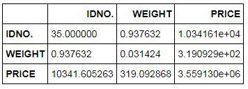
Covariance Matrix

Covariance is a measure of correlation (note that the correlation coefficient is a scaled form of covariance, thus we get Correlation Coefficients when we standardize the covariance) and has been mentioned in the theoretical blog of Correlation Coefficients. We can calculate the covariance matrix by using the following command in Python.

DiamondData.cov()

Chi-Square Test

Import Dataset: Unlike Correlation Coefficients, Chi-Square is used to test the level of association between two categorical variables. To perform a chi-square test in Python, we use a hypothetical dataset where we have two categorical variables, Gender and Smoke.

SmokeData = pd.read_excel("C:/Users/user/Desktop/Data Sets/SmokingData.xls")
SmokeData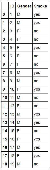

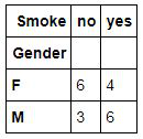
Show full table ▾

Frequency Table

In the blog, Chi Square under the theory section (where the chi-square value is calculated without the use of any application), the need and importance of a frequency table has been explored. Here in Python also, we first create a frequency table using both the categorical variables.

Smoke_table = pd.crosstab(index=SmokeData["Gender"],columns=SmokeData["Smoke"])
Smoke_table

Running Chi-Square Test

Our objective is to find if there is any relation between Gender and the habit of Smoking, and as both are categorical variables, we perform a chi-square test where our null hypothesis is that these two variables are independent (not related) of each other.

chi2, p, ddof, expected = scipy.stats.chi2_contingency(Smoke_table)
msg = "Test Statistic: {}\np-value: {}\nDegrees of Freedom: {}\n"
print( msg.format( chi2, p, ddof ) )
print( expected )

The p-value comes out to be 0.4825126366316421 and as the p-value is greater than 0.05, therefore, we fail to reject the null hypothesis, i.e. there is no statistically significant association between the two variables.

In this blog, we applied the concepts explored in the theory part of Inferential Statistics. Python is a powerful tool and can be used for bivariate analysis using various inferential statistics. Various bivariate analyses can be performed that have been explored in Descriptive Statistics in Python and can be put to use to better understand the data. In the next section, Python will be used to apply the various concepts of data preparation explored in section two of Theory - Data Exploration and Preparation.