// application · r
Inferential Statistics in R
Inferential statistics are used to draw inferences from the sample of a huge data set. Random samples of data are taken from a population, which are then used to describe and make inferences and predictions about the population. In the Theory section, various Inferential Statistics were explored and in this blog, all those inferential statistics will be put to use using R.
In this section, the following topics will be explored:
- Z Scores & Z-Test
- t-Tests
- F-test
- Correlation Coefficients
- Chi-Square
Z Scores, Z-Test
Z-Scores are used to calculate the probability of a score occurring within our normal distribution. This helps us to compare scores of two or more different normal distributions.
Z Value
Import Dataset: We import a hypothetical data set having exam scores of students.
Z_ScoresData <- read_excel("C:/Users/user/Desktop/Data Sets/Marks_Scored.xls")
View(Z_ScoresData)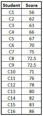
Calculating Z Score
The following codes can be used to compute Z scores. As there is no inbuilt function to calculate z scores, therefore we will first calculate the parameters such as population standard deviation, population mean etc.
Population Standard Deviation.
Scores <- Z_ScoresData$Score
pop_sd <- sd(Scores)*sqrt((length(Scores)-1)/(length(Scores)))
pop_sd
Population Mean.
pop_mean <- mean(Scores)
pop_mean
Z Score.
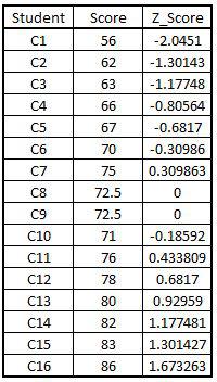
Z_Score <- (Scores-pop_mean)/pop_sd
Z score in Dataset: We now combine the calculated z scores column with our dataset.
New_ZScoreData <- cbind(Z_ScoresData,Z_Score)
Exporting the Data.
write.csv(New_ZScoreData,"C:/Users/user/Desktop/Data Sets/New_ZScore.csv")
Finding Percentage / Area Under the Curve
We can find out the percentage of people who scored above 70. We take the mean and standard deviation to calculate the area under the curve. Here we use the following code for finding the area under the curve, to find the percentage of students who scored more than 70 marks.
Plessthan70 <- pnorm(70,pop_mean,pop_sd)
Plessthan70
Finding the area of students score>70.
Pmorethan70 <- 1-Plessthan70
Pmorethan70
62.16% people scored more than 70 marks.
Z Test
Z-test is used to test whether the two datasets are similar or not.
Import Dataset: We take a population dataset and a random sample of the population dataset. We first import the population dataset.
Height1 <- read.csv("C:/Users/user/Desktop/Data Sets/Heightof200ppl.csv")
mean(Height1$Height..in.cm.)We now import a sample dataset.
HeightSample <- read_excel("C:/Users/user/Desktop/Data Sets/HeightDataSample.xls")
var(HeightSample$`Height(in cm)`)Performing Z Test: Again, there is no inbuilt function in R for Z test, therefore we will create the function by running the following code in the editor window. This function will be saved in the global environments and can be used for other datasets also. Here we will make use of the mean of the population and variance of the sample dataset to see if the two datasets are significantly similar or not.
z.test = function(a,mu,var){
  zeta=(mean(a)-mu)/(sqrt(var/length(a)))
  return(zeta)
}
After creating the function, we will calculate the Z statistic for the sample data.
a<- HeightSample$`Height(in cm)`
z <- z.test(a,164.075,93.60324)
We will now calculate the p-value from the z statistic to decide if our null hypothesis is true or not.
p_value <- 2*pnorm(-abs(z))
In the output, we get the Z Statistic to be at -1.190425 while the p-value comes out to be 0.2338793. As discussed in Z scores, Z test and Probability Distribution, our null hypothesis in this scenario will be that both the datasets are significantly similar. If we consider the significance level to be at 5%, then to accept the null hypothesis, our p-value should be more than the chosen significance level. In our example, the p-value is well above 0.05 (5%) thus the Z-Test correctly indicates that the means of both the datasets are the same and are not statistically significantly different from each other.
t-Test
t-Test is used to see whether two groups are similar or not. Z-test is also used for the same purpose, however, the difference between these tests is that the Z-test is used when the sample size is greater than 30, whereas t-Test is used when the sample size is less than 30. The difference has been explored in Brief Intro to T Test. There are different types of t-Tests for different scenarios and we put them to use below.
Two-sided One-Sample t-Test
Import Dataset: We will be working on a hypothetical Diamond dataset which has the information of the diamonds that were sold in a shop.
DiamondData <- read_excel('C:/Users/user/Desktop/Data Sets/DiamondData.xls')
View(DiamondData)
Perform Two-Tailed t-Test: We perform a One-Sample t-Test where we try to find that whether the mean of the variable 'WEIGHT' is statistically greater than 0.5 or not. Since this is a two-sided one-sample t-test, our Null Hypothesis is that the mean of 'WEIGHT' equals 0.5, and the Alternative Hypothesis is that it is not equal to 0.5. We now run a One-Sample t-Test to test this hypothesis.
t.test(DiamondData$WEIGHT,mu=0.5,alternative="two.sided")
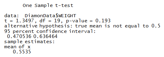
Unlike Python, R gives the value of mean in the output of t-test itself and we don't have to calculate it separately.
In our case the p-value comes out to be 0.193 which is greater than 0.05 (5% significance level) therefore, we fail to reject the null hypothesis that the mean equals 0.5; the difference from 0.5 is not statistically significant.
Independent t-Test
Import Dataset: Here we import an arbitrary, hypothetical dataset that has ID, age and their gender as variables.
AgeData = read.csv("C:/Users/user/Desktop/Data Sets/data1.csv")
View(AgeData)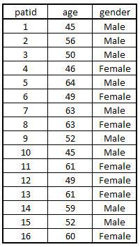
Our Null hypothesis is stated as below:
H0: Mean of Age for Males and Females are significantly similar.
Running Independent t-Test: We run an Independent t-Test using the function t.test. For independent t-test we mention var.eq = False(F) to specify for independent test. Var.eq is used to tell the program whether the variables have equal variance or not.
t.test(AgeData$age~AgeData$gender,mu=0,alt="two.sided",var.eq=F)
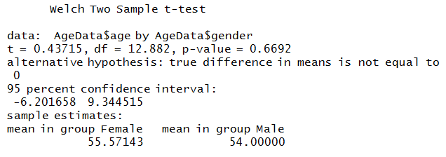
Our null hypothesis is that both groups are statistically significantly similar. Here, the p-value is greater than 0.05, therefore, we accept the null hypothesis that these two groups are significantly similar. Even though the sample means differ, the difference between them is not statistically significant and can be attributed to sampling error.
Paired t-Test
Import Dataset: We import a hypothetical dataset that has marks of students in two different tests. Here we presume that they are the same tests undertaken over a period of time.
ScoresData =read_excel("C:/Users/user/Desktop/Data Sets/Student Test Scores.xls")
View(ScoresData)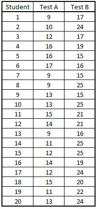
Running Paired t-Test: We need to find whether the marks/score of the students have changed over time or not. For this, we compare the mean of the two tests and see if they are statistically significantly different from each other or not. Here our null hypothesis is that both test scores are significantly similar.
t.test(ScoresData$`Test A`,ScoresData$`Test B`,mu=0,alternative = "two.sided",paired = T)
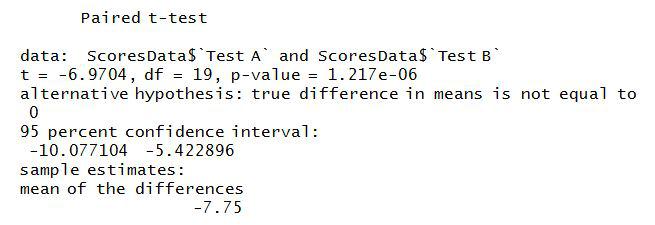
We find that the p-value comes out to be 1.217e-06 which is very less than 0.05 (significance level of 5%). Therefore, we reject the null hypothesis i.e. these test scores are significantly different from each other.
F-test
Different types of F-Tests have been discussed under the theoretical blog for F-Tests, however, the most common F test is One-Way ANOVA. We can use the Age data used in the Independent t-Test and find if the age of males and females is statistically significantly different from each other or not.
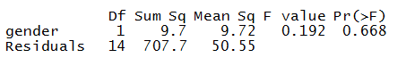
ANOVA1 <- aov(age~gender,data=AgeData)
ANOVA1
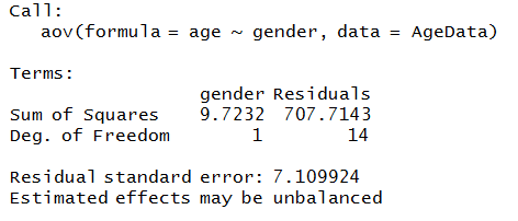
We now use the summary command.
summary(ANOVA1)
Correlation Coefficients
Import Dataset: To come up with correlation coefficients, we used the diamond dataset that we have used above for performing Two-Tailed t-Test.
DiamondData <- read_excel('C:/Users/user/Desktop/Data Sets/DiamondData.xls')
View(DiamondData)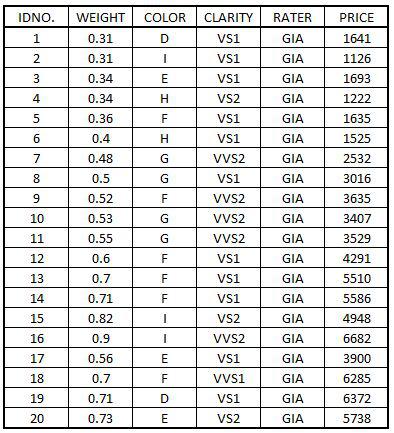
Scatter Plot
We create a scatterplot to study the correlation between two variables. In this example we chose two variables 'WEIGHT' and 'PRICE' from our Diamond dataset.
plot(DiamondData$WEIGHT,DiamondData$PRICE,main="Scatter Plot for Correlation",xlab="weight",ylab="Price")
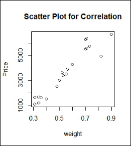
The scatterplot shows a positive correlation between the two variables and thus there is a direct relation between Price and Weight of the diamond. An increase in weight will correspond to an increase in the Price of that diamond.
Calculating Correlation Coefficient
If we need to properly quantify the relationship between the two variables then rather than going for a visual approach, we are required to calculate correlation coefficient. We do this by using a function called cor.
cor(DiamondData$WEIGHT,DiamondData$PRICE)
Correlation Coefficient Matrix
If we have a lot of variables then rather than calculating the correlation coefficient for each combination of variables we can come up with Correlation Coefficient Matrix. Here all the diagonal values will be 1 while correlation coefficient will be there for all the combination of the numerical variables. There are two methods of calculating Correlation Coefficient and its matrix - Pearson and Spearman.
Pearson correlation coefficient: Correlation Coefficient matrix using Pearson's method.
cor(DiamondData[c('IDNO.','WEIGHT','PRICE')], use="complete.obs", method="pearson")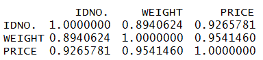
Spearman correlation coefficient: Correlation Coefficient matrix using Spearman's method.
cor(DiamondData[c('IDNO.','WEIGHT','PRICE')], use="complete.obs", method="spearman")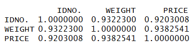
Covariance Matrix
Covariance is a measure of correlation (Note that the correlation coefficient is a scaled form of covariance thus we get Correlation Coefficients when we standardize the covariance) and has been mentioned in the theoretical blog of Correlation Coefficients.
cov(DiamondData[c('IDNO.','WEIGHT','PRICE')], use="complete.obs")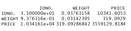
Chi-Square Test
Import Dataset: Unlike Correlation Coefficients, Chi-Square is used to test the level of association between two categorical variables. To perform a chi-square test in R, we use a hypothetical dataset where we have two categorical variables Gender and Smoke.
SmokeData <- read_excel('C:/Users/user/Desktop/Data Sets/SmokingData.xls')
View(SmokeData)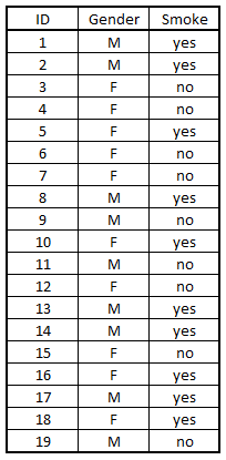
Frequency Table
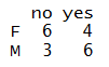
In the blog, Chi Square under the theory section, (where the chi-square value is calculated without the use of any application), the need and importance of frequency table has been explored.
table2 <- table(SmokeData$Gender,SmokeData$Smoke)
table2
Running Chi-Square Test
Our objective is to find if there is any relation between Gender and the habit of Smoking and as both are categorical variables, we perform a chi-square test where our null hypothesis is that these two variables are independent (not related) of each other.
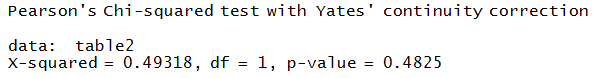
CHI <- chisq.test(table2,correct = T)
CHI
We now use the attribute command.
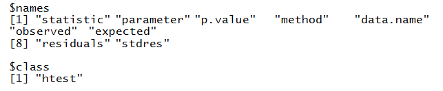
attributes(CHI)
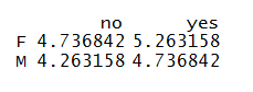
We can now come up with the expected table as explored in the theory section.
CHI$expected
The p-value comes out to be 0.48251 and as the p-value is greater than 0.05 therefore, we fail to reject the null hypothesis, i.e. there is no statistically significant association between the two variables.
In this blog, we applied the concepts explored in the theory part of Inferential Statistics. R is a powerful tool and can be used for bivariate analysis using various inferential statistics. Various bi-variate analysis can be performed that have been explored in Descriptive Statistics in R and can be put to use to better understand the data. In the next section, R will be used to apply the various concepts of data preparation explored in section two of Theory - Data Exploration and Preparation.